User Guide and Examples
Processing of a “raw” 1D spectrum
Let us say that your spectrum is saved in the folder /home/myself/spectra/mydataset/1/. Initialize the spectrum object through:
Path = r"/home/myself/spectra/mydataset/1/"
s = Spectrum_1D(Path)
This command will do three main tasks:
read the binary FID of your spectrum and store it in a complex array
s.fid;load the acquisition parameters, read the interesting keys and store them in a dictionary
s.acqus;initialize a dictionary
s.procswhich contains the processing parameters.
KLASSEZ is able to read also Varian and Spinsolve (Magritek) data,
by specifying the option “spect”.
A detailed description of acqus and procs is shown in
Table 1 and Table 2.
Please note that reading the spectrum causes the program to save a file called “name.procs”, where “name” is the path name.
Key |
Explanation |
|---|---|
|
Magnetic field strength /T |
|
Spectrometer format: |
|
Endianness of binary data: |
|
Binary data type: |
|
Number of points of the digital filter |
|
Observed nucleus |
|
Carrier frequency i.e. center of the spectrum, in ppm |
|
Same as |
|
Sweep width, in ppm |
|
Sweep width, in Hz |
|
Larmor frequency of the observed nucleus at field
|
|
Number of sampled complex points |
|
Dwell time, i.e. the sampling interval, in seconds |
|
Time duration of the FID |
|
Acquisition timescale |
Key |
Explanation |
|---|---|
|
Window function. This is a dictionary itself:
|
|
Zero-filling. Set the final number of points! |
|
Number of points to be used for processing |
|
Scaling factor for the first point of the FID before Fourier transform |
|
Frequency-independent phase correction /degrees |
|
First order phase correction /degrees |
|
Pivot point for the first order phase correction /ppm |
|
Set of coefficients of a polynomion to be used as baseline, starting from the \(0\)-order coefficient |
|
Offset, in ppm, to be added to the frequency and ppm scales for calibration |
To make the Fourier transform of the FID to obtain the spectrum, you
must invoke the klassez.Spectra.Spectrum_1D.process() method, which reads the procs dictionary
to get the instructions on the processing you want to make on your
spectrum. For instance, if you want to obtain a final spectrum of
\(8k\) points with an exponential broadening of 25 Hz:
s.procs["wf"]["mode"] = "em"
s.procs["wf"]["lb"] = 25
s.procs["zf"] = 8192
s.process()
s.pknl()    # Tries to remove the digital filter through a first-order phase correction
It is also possible to use composite functions by combining more methods. For instance:
s.procs["wf"]["mode"] = "em", "qsin"
s.procs["wf"]["lb"] = 10, 0
s.procs["wf"]["ssb"] = 0, 2
will generate a composite window function made with em, lb=10 and qsin, ssb=2.
Calling the klassez.Spectra.Spectrum_1D.process() method generates new attributes of the class:
self.freq: the frequency scale, in Hz;self.ppm: the ppm scale;self.r: the real part of the spectrum;self.i: the imaginary part of the spectrum;self.S: the complex spectrum (\({\tt S} = {\tt r} + \ui {\tt i}\)).
After the Fourier transform, the klassez.Spectra.Spectrum_1D.process() method applies the phase
correction and the calibration using the phase angles and the
calibration value saved in the procs dictionary automatically. This
allows the user to not phase their spectra every time, as well as
keeping a record of the processing.
If the spectrum requires phase correction, you can perform it interactively (Figure 1):
s.adjph()
or by passing the phase angles, in degrees, to adjph(). Example, if
you know you need to phase your spectrum with \(30\) degrees of
\(\phi^{(0)}\) and \(-55\) degrees of \(\phi^{(1)}\) with
the pivot set at 7.32 ppm:
s.adjph(p0=30, p1=-55, pv=7.32)
In both cases, the phase angles are updated in the procs dictionary.
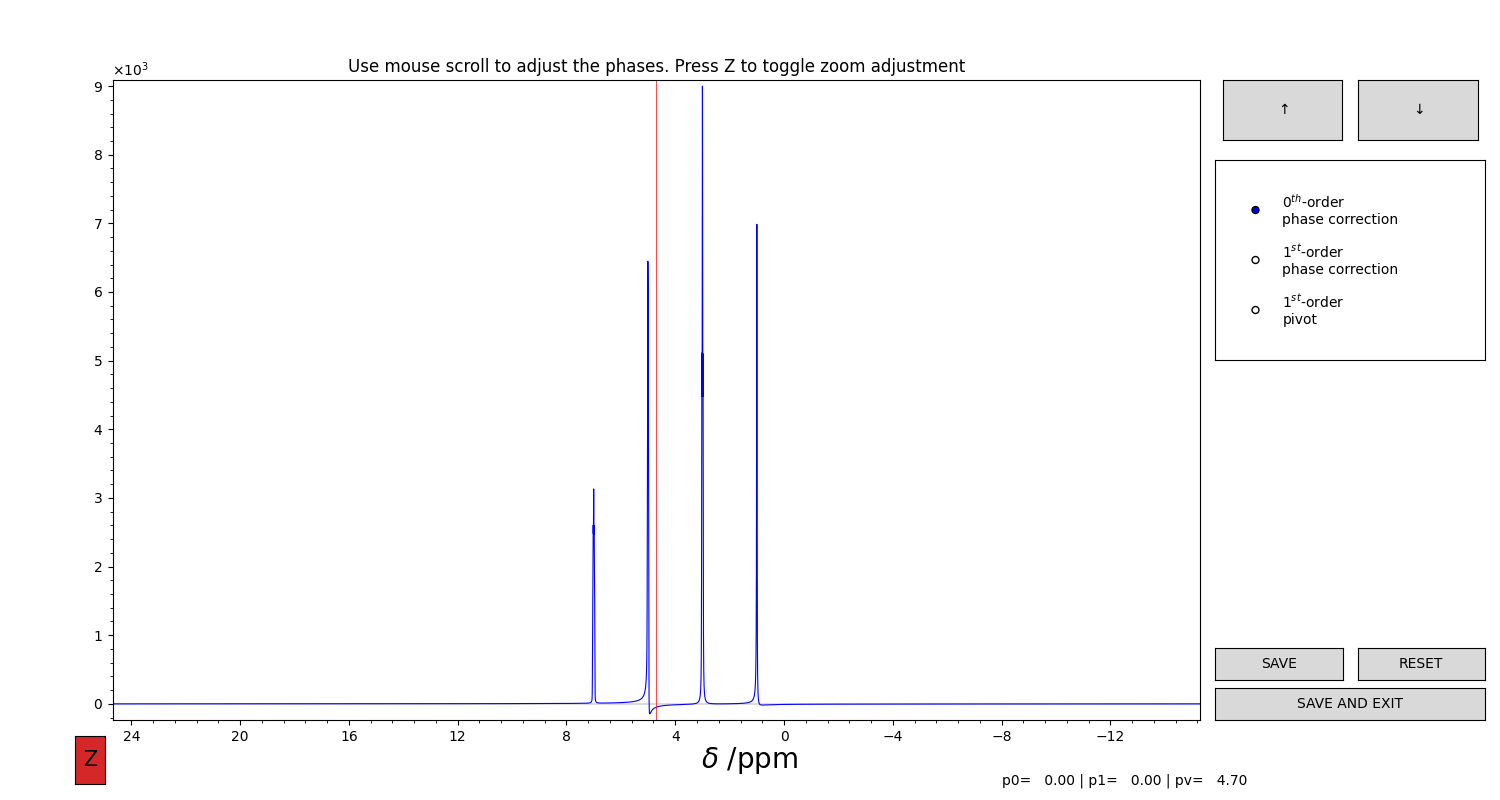
Figure 1 GUI for the interactive phase correction of a 1D spectrum. You can select the value to modify (0, 1st order or pivot) from the selector on the right. Then, use the mouse scroll to edit the values. The arrow buttons at the top increase or decrease the sensitivity of the movement. Press “Z” on the keyboard to toggle the automatic adjustment of the vertical limits. Press “SAVE” to save the results of the phasing.
The spectrum can be calibrated by using a dedicated GUI (Figure 2).
To do so, you must call for the method klassez.Spectra.Spectrum_1D.cal() with the option from_procs=False.
The option from_procs=True (default) will only apply the values stored in self.procs['cal'].
s.cal(from_procs=False)
Alternatively, you can specify the shift value in ppm or in Hz (in this case, be sure to
set the isHz keyword to True).
s.cal(-3)               # Shift of -3 ppm
s.cal(1000, isHz=True)  # Shift of +1 kHz
Both ppm and freq are updated according to the given values.
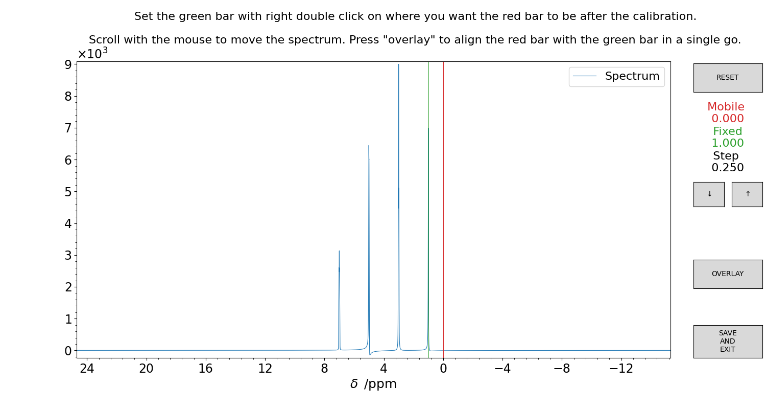
Figure 2 GUI for the interactive calibration of a 1D spectrum. The green bar moves together with the spectrum, the red bar is the reference. First, set the green bar with right-double-click of the mouse on a reference signal. Then, set the red bar with left-double-click on the final, calibrated position on the ppm scale. Now, use the mouse scroll to move the spectrum, or click on the “OVERLAY” button to teleport the green position on the red. The values are written on the right side of the figure panel. Press “SAVE” to store the result.
Another sometimes useful feature is the possibility to remove one signal from the spectrum (usually, the solvent resonance).
To do so, there is the klassez.Spectra.Spectrum_1D.qfil() method.
s.qfil()
The idea is to apply a reverse-gaussian filter (i.e. a V-shaped function that is 1 everywhere and goes to 0 at a given position, smoothly as a Gaussian),
with the position in ppm and the width in Hz.
When invoked, the function will first look into the procs dictionary to see if there is a 'qfil' key. If it exists, the function computes the filter
and applies it without further questions. Otherwise, it opens a GUI for the visual optimization of the parameters, which is shown in Figure 3.
If the option from_procs=False is passed, the GUI is opened anyways and the final values are overwritten.
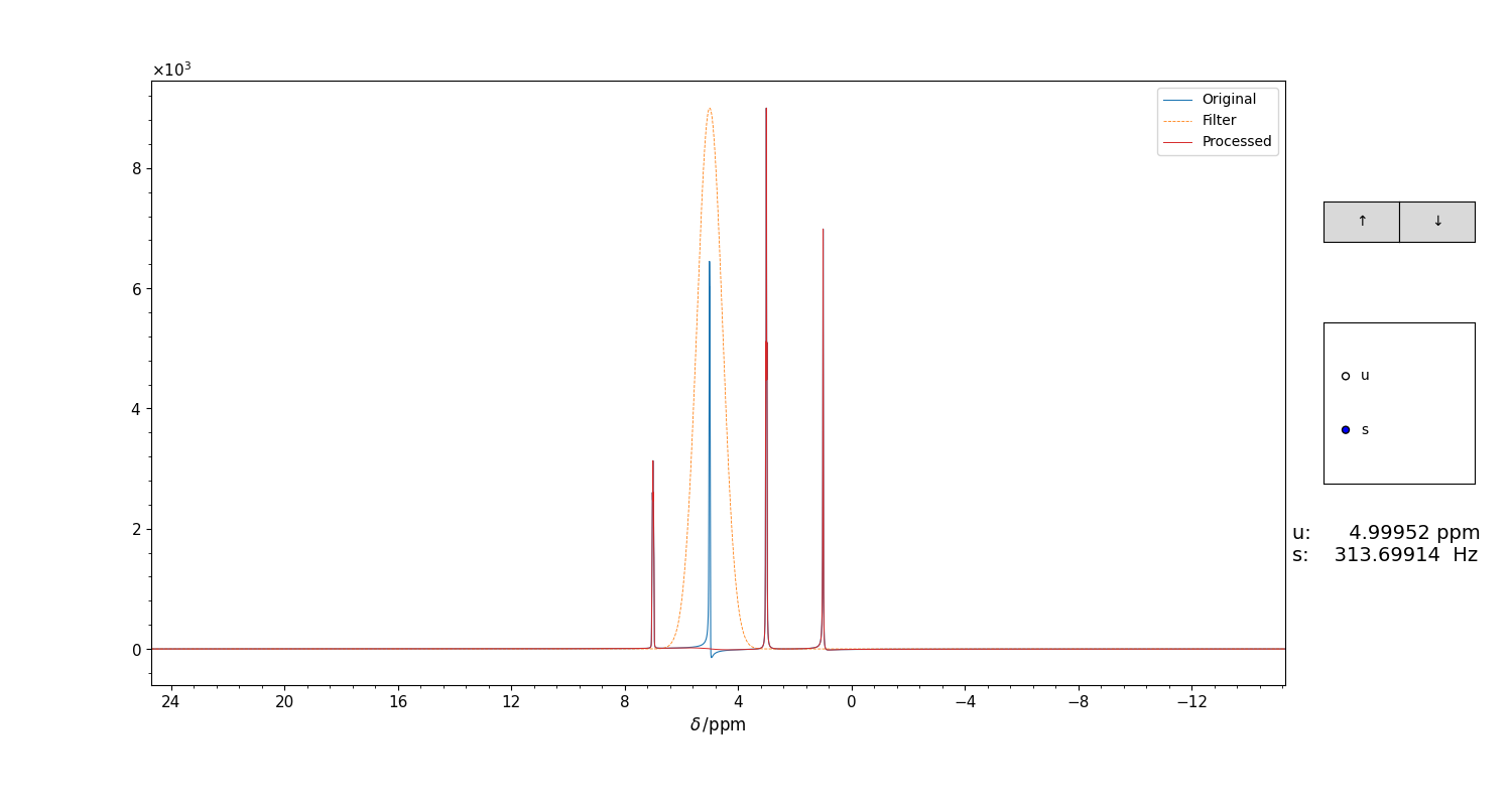
Figure 3 GUI for the selection of the parameters for the gaussian filter for klassez.processing.qfil(), which is invoked by the qfil() of the Spectra classes.
The filter appears, upside down, as an orange trace. The original spectrum appears in blue, the spectrum after the filtering is displayed in real time in red.
Use the mouse scroll to adjust the values (which appear under the selector box). Close the figure to save the parameters.
It is also possibile to pass the values of the filter from outside, without passing for the GUI:
u = 5.0     # chemical shift of the signal to suppress
s = 310     # standard deviation of the filter in Hz
s.qfil(u=u, s=s)
The filter is applied directly on the real part of the spectrum only. The imaginary part is automatically reconstructed via Hilbert transform. Therefore, if you want to perform further processing, be sure to have zero-filled the FID to at least twice its original size, otherwise you will get errors!
The class pSpectrum_1D
The class Spectrum_1D does not work if you want to read the
processed data directly from TopSpin (or whatever software you used to
acquire and process them). Instead, you should use the class
klassez.Spectra.pSpectrum_1D, which is designed to perform exactly this task. It
inherits most of the attributes and methods of the klassez.Spectra.Spectrum_1D
class, therefore its usage closely resembles the example reported in the
previous section.
Processing of a “raw” 2D spectrum
Let us say that your spectrum is saved in the folder /home/myself/spectra/mydataset/21/. Initialize the spectrum object through:
Path = r"/home/myself/spectra/mydataset/21/"
s = Spectrum_2D(Path)
The generated acqus and procs dictionaries include informations
on both dimensions.
Key |
Explanation |
|---|---|
|
Magnetic field strength /T |
|
Endianness of binary data: |
|
Binary data type: |
|
Number of points of the digital filter |
|
Observed nucleus in the indirect dimension |
|
Observed nucleus in the direct dimension |
|
Carrier frequency i.e. center of the indirect dimension, in ppm |
|
Carrier frequency i.e. center of the direct dimension, in ppm |
|
Same as |
|
Same as |
|
Sweep width of the indirect dimension, in ppm |
|
Sweep width of the direct dimension, in ppm |
|
Sweep width of the indirect dimension, in Hz |
|
Sweep width of the indirect dimension, in Hz |
|
Larmor frequency of the observed nucleus in F1 at
field |
|
Larmor frequency of the observed nucleus in F2 at
field |
|
Number of \(t_1\)-increments |
|
Number of sampled complex points |
|
\(t_1\) increments, in seconds |
|
Dwell time, i.e. the sampling interval, in seconds |
|
Sampled timescale of the indirect dimension |
|
Time duration of the FID |
|
Evolution timescale |
|
Acquisition timescale |
Key |
Explanation |
|---|---|
|
Window function. This is a dictionary itself:
|
|
Zero-filling. Set the final number of points! |
|
Number of points to be used for processing |
|
Scaling factor for the first point of the FID before Fourier transform |
|
Frequency-independent phase correction /degrees, direct dimension |
|
First order phase correction /degrees, direct dimension |
|
Pivot point for the first order phase correction /ppm, direct dimension |
|
Frequency-independent phase correction /degrees, indirect dimension |
|
First order phase correction /degrees, indirect dimension |
|
Pivot point for the first order phase correction /ppm, indirect dimension |
|
Calibration offset for F1 /ppm |
|
Calibration offset for F2 /ppm |
Then, the sequence of commands for the processing resembles the ones of the 1D spectra.
s.process()
s.pknl()    # Remove the digital filter
# Also in this case, phase correction and calibration are performed automatically with the values in procs
s.adjph()
s.plot()
The keys for adjph are of the kind: pXY, where X is the
order of the phase correction (\(0\) or \(1\)) and Y is the
dimension on which to apply it (\(1\) or \(2\)). Explicative
table below:
F1 |
F2 |
|
|---|---|---|
\(\phi^{(0)}\) |
|
|
\(\phi^{(1)}\) |
|
|
pivot |
|
|
The GUI for the interactive phase correction on 2D spectra works in two steps. First, you have to select the traces to use as probes for the phase of the spectrum (Figure 4). Then, you can proceed to the actual phasing (Figure 5).
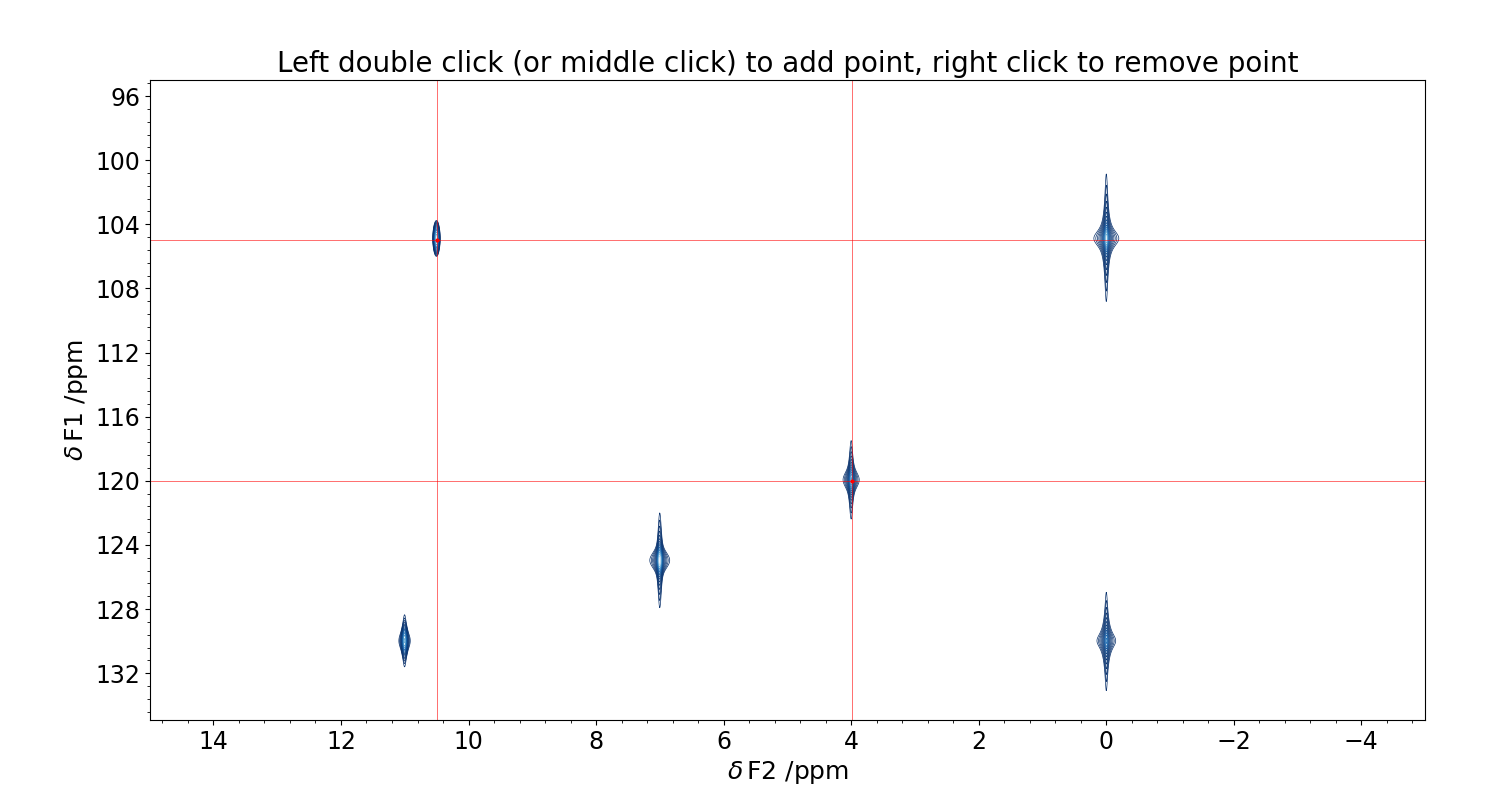
Figure 4 GUI for the selection of the traces to be used for the phase correction. Double click with the mouse where you want to compute the projection, and a red crossmark will appear. To remove an existing marker, align the cursor with it and click with the right button of the mouse. Use the scroll to adjust the contour levels. Close the figure to save.
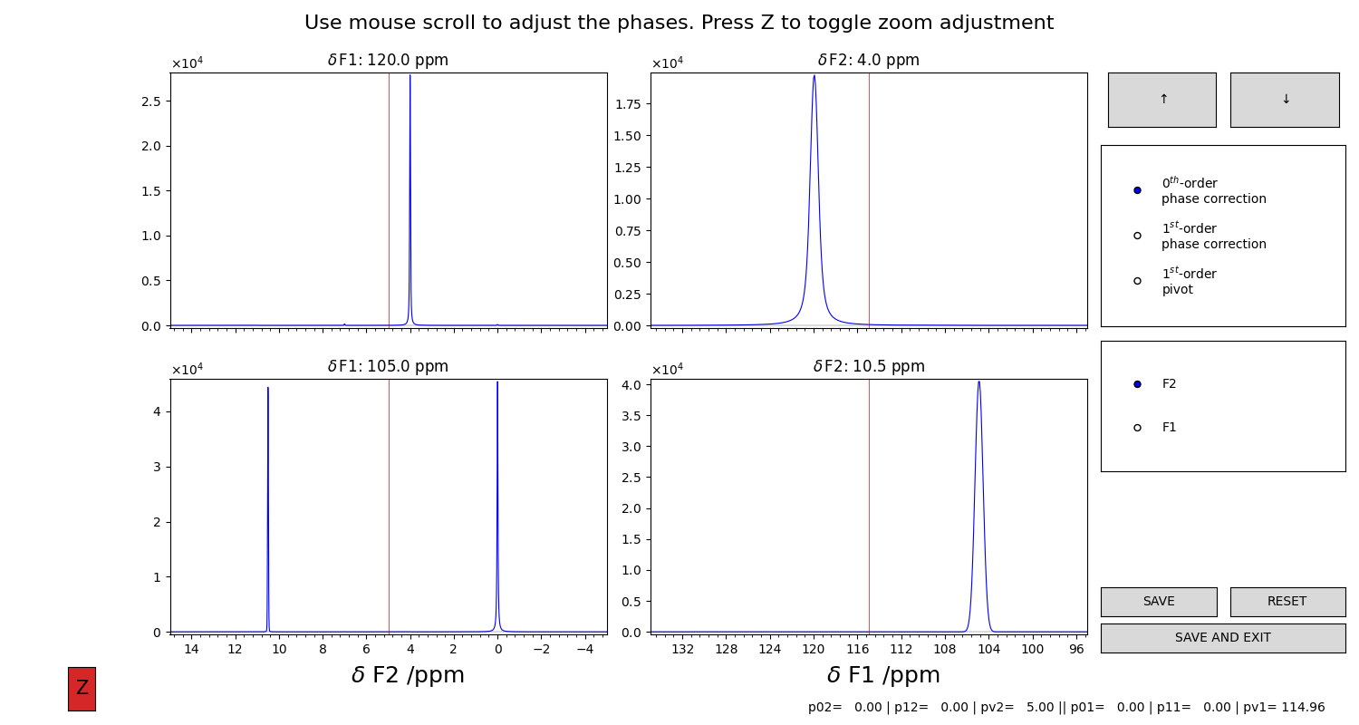
Figure 5 Here, the projections computed as in Figure 4 are drawn in this plot. The projection on the direct dimension are in the left column, the ones of the indirect dimension are in the right column. Use the selector and the mouse scroll to change the values of the parameters. You will see all the traces to change in response of your actions. Press “SAVE AND CLOSE” to save the processed spectrum.
The calibration of a 2D spectrum works as in the 1D case, using the klassez.Spectra.Spectrum_2D.cal() method.
For the interactive calibration, you will be prompted to select a reference trace
by using the same GUI of Figure 4. Then you will calibrate one dimension at the time with the GUI in Figure 2.
s.cal()
If you are sure that you want to calibrate only one dimension, there exist wrapper methods:
s.calf2()
s.calf1()
On the processed data, one may want to use the method qfil() to suppress the solvent signal.
This can be done interactively by invoking the function without further arguments:
s.qfil()
The function works exactly as the 1D counterpart. However, the GUI will first ask you to select a trace to use
as reference for the computation of the filter, which is applied in a ridge-like manner on the whole 2D spectrum.
The imaginary parts are reconstructed via Hilbert transform, hence be sure to have zero-filled enough!
The key qfil = {'u': u, 's': s} are then saved in the procs dictionary for additional use.
If these keys are present in the procs dictionary, the filtering is applied without prompting for the GUI, unless
from_procs=False.
Another useful option is to make a so-called “strip transform” to use only the part of the spectrum you are interested in. Example:
xlim = (max(s.ppm), 6)
ylim = None
s.strip(xlim=xlim, ylim=ylim)
will trim the direct dimension from the left side of the spectrum to 6 ppm, and leave the indirect dimension untouched.
To read the processed data, use the pSpectrum_2D class instead.
Computing projections
While the 2D spectra give an overall look on the whole experiment, the
user might want to extract projection of the direct or the indirect
dimension, to focus onto particular features in the spectrum. In order
to do so, KLASSEZ offers two commands: projf1 and projf2,
which compute the sum projections on the indirect or on the direct
dimension, respectively, and store the result in dictionaries called
trf1 and trf2, whose keys are the ppm values correspondant to
the projections. Actually, the capitalized versions of the two
dictionaries (with the same keys), i.e. Trf1 and Trf2, can be
more useful, as they are instances of the pSpectrum_1D class and
therefore are initialized with ppm scales and other parameters.
Example:
# Supposed to have a 1H-15N HSQC spectrum

#   Extract the direct dimension trace at 115 ppm, 15N scale
s.projf2(115)
#   Access to it through
Proj_115 = s.Trf2['115.00']

#   Extract the indirect dimension trace from 6 to 8 ppm, 1H scale
s.projf1(6, 8)
Proj_indim = s.Trf1['6.00:8.00']

# You can plot them:
Proj_115.plot()
Proj_indim.plot()
Simulating data
The classes Spectrum_1D and Spectrum_2D are also able to
generate simulated data by reading a custom-written input file. The
functions they use are klassez.sim.sim_1D() and klassez.sim.sim_2D().
Simulate 1D data
The input file you have to write must have the following keys:
B0: Magnetic field strength /T;nuc: Observed nucleus (e.g.13C);o1p: Carrier frequency i.e. centre of the spectrum /ppm;SWp: Sweep width /ppm. The spectrum will cover the range \([{\tt o1p} - {\tt SWp}/2, {\tt o1p} + {\tt SWp}/2]\);TD: Number of sampled (complex) points;shifts: sequence of peak positions /ppm;fwhm: Full-width at half-maximum of the peaks /Hz;amplitudes: Intensity of the peaks in the FID;b: Fraction of gaussianity. \(\beta = 0 \implies\) pure Lorentzian peak, \(\beta = 1 \implies\) pure Gaussian peak;
and can have the following keys:
phases: phases of the peaks /degrees. Default: all zeros;mult: fine structures of the peaks (e.g. doublets of triplets:dt). Default: all singlets;Jconst: coupling constants of the fine structures /Hz. If more of one coupling is expected, provide them as a sequence. Default: not used as the peaks are all singlets.
Key and value must be separated by a tab character. You are allowed to
leave empty rows to improve the readibility and to insert comments using
the # character.
Example:
B0          16.4    # 700 MHz 1H
nuc         1H
o1p         4.7
SWp         40
TD          8192

shifts      1, 3, 5, 7
fwhm        [10 for k in range(4)]
amplitudes  10, 20, 15, 10
b           0, 0.4, 0.6, 1
phases      5, 0, 10, 0

mult        s, t, dt, ddd
Jconst      0, 15, [12, 9.5], [25, 15, 10]
This input file generates the spectrum in Figure 6.
Code:
#! /usr/bin/env python3

from klassez import *

s = Spectrum_1D('sim_in_1D', isexp=False)
s.process()

figures.figure1D(s.ppm, s.r, name='test_1D', X_label=r'$\delta\, ^1$H  /ppm', Y_label=r'Intensity /a.u.')
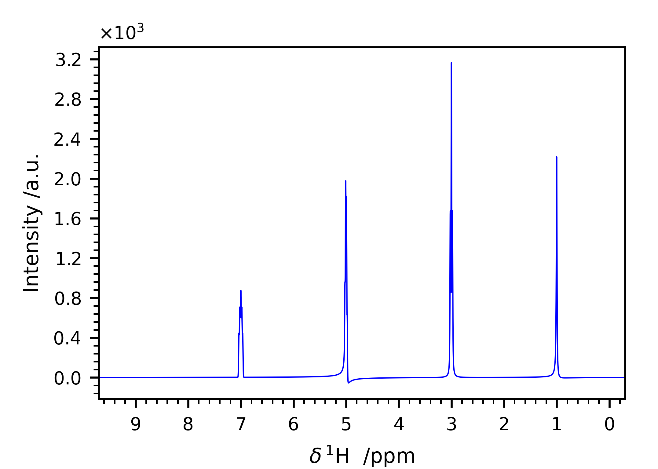
Figure 6 Simulated spectrum with the input file shown in Listing 1.
Simulate 2D data
The same procedure can be followed to simulate 2D spectra. The input file to write is very similar to the one for 1D data, except for the quantities that clearly span over two dimensions. As in NMR textbook, the direct and indirect dimensions will be named F2 and F2 respectively, and dimension-specific quantities will feature the 1 or 2 labels accordingly.
B0: Magnetic field strength /T;nuc1: Observed nucleus in F1(e.g.13C);nuc2: Observed nucleus in F2(e.g.1H);o1p: Carrier frequency i.e. center of F1 /ppm;o2p: Carrier frequency i.e. center of F2 /ppm;SW1p: Sweep width /ppm. The indirect dimension will cover the range \([{\tt o1p} - {\tt SW1p}/2, {\tt o1p} + {\tt SW1p}/2]\);SW2p: Sweep width /ppm. The direct dimension will cover the range \([{\tt o2p} - {\tt SW2p}/2, {\tt o2p} + {\tt SW2p}/2]\);TD1: Number of sampled (complex) points in F1;TD2: Number of sampled (complex) points in F2;shifts_f1: sequence of peak positions in F1 /ppm;shifts_f2: sequence of peak positions in F2 /ppm;fwhm_f1: Full-width at half-maximum of the peaks in F1 /Hz;fwhm_f2: Full-width at half-maximum of the peaks in F2 /Hz;amplitudes: Intensity of the peaks in the FID;b: Fraction of gaussianity. \(\beta = 0 \implies\) pure Lorentzian peak, \(\beta = 1 \implies\) pure Gaussian peak;
Phase distortions and fine structures are not allowed for multidimensional spectra. The indirect dimension will be generated employing the States-TPPI sampling scheme.
Example:
B0           28.2
nuc1         15N
nuc2         1H
o1p          115
o2p          5
SW1p         40
SW2p         20
TD1          256
TD2          2048

shifts_f1    130.0, 105.0, 120.0, 1.25e2, 130.0, 105.0
shifts_f2    0.0, 0.0, 4.0, 7.0, 1.1e1, 10.5
fwhm_f1      100, 100, 100, 100, 100, 100
fwhm_f2      50, 50, 50, 50, 50, 50
amplitudes   10, 20, 10, 20, 10, 10
b            0.0, 0.2, 0.4, 0.6, 0.8, 1.0
This input file generates the spectrum in Figure 7.
Code:
#! /usr/bin/env python3

from klassez import *

s = Spectrum_2D('sim_in_2D', isexp=False)
s.process()

figures.figure2D(s.ppm_f2, s.ppm_f1, s.rr, lvl=0.005, name='test_2D', X_label=r'$\delta\, ^1$H  /ppm', Y_label=r'$\delta\, ^{15}$N  /ppm')
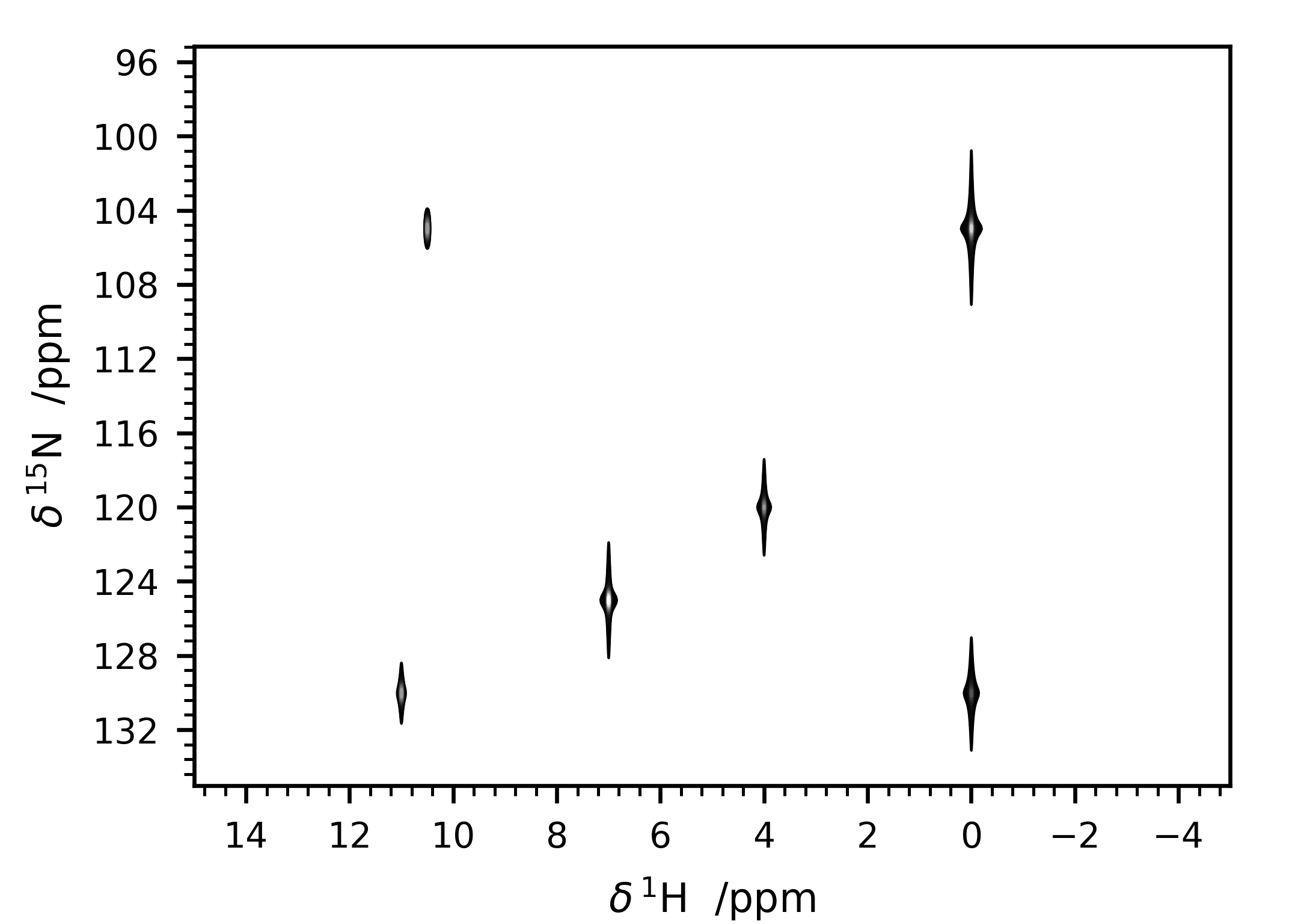
Figure 7 Simulated 2D spectrum with the input file shown in Listing 2.
Processing of a “raw” pseudo-2D spectrum
“Classic” pseudo-2D processing
Sometimes, the spectroscopist might find interesting to acquire a series of 1D experiments in which one (or more) parameters are changed according to a certain schedule. This kind of experiments are 2D in principle, but their processing and analysis resemble the one of 1D spectra. Therefore, they lie somewhere in between 1D spectra and 2D spectra, hence they are often referred to as pseudo_2D.
Also in this case, KLASSEZ offers a specific class to deal with this
kind of data: klassez.Spectra.Pseudo_2D. Pseudo_2D is a subclass of
Spectrum_2D; however, many functions have been adapted to resemble
the 1D version.
Pseudo_2D does not encode for a routine to automatically simulate
data. If you want to, you should give a 1D-like input file (just like
the one in the previous section), and replace the attribute
fid with your FID by using the method mount(), generated as you
wish. With a real dataset this is not required, as it is able to read
everything automatically.
path_to_pseudo = "/home/myself/spectra/mydataset/899/"
s = Pseudo_2D(path_to_pseudo)
The process() function applies apodization, zero-filling and Fourier
transform only on the direct dimension, reading the parameters from a
procs dictionary like the one of Spectrum_1D. The attributes
freq_f1 and ppm_f1 are initialized with
np.arange(N), where N is the number of
experiments that your FID comprises of. In particular, freq_f1
numbers the experiments sequentially from \(0\) to \(N-1\),
whereas ppm_f1 does it from \(1\) to \(N\). Therefore, when
calling the method projf2 to extract the experiments as
Spectrum_1D objects, the argument must follow ppm_f1. As an
example, to project the first transient, one should type
s.projf2(1)
and access to it from
t = s.Trf2["1.00"]
The user can replace this “standard” numbering with the actual parameter
that is varied during the evolution of the indirect dimension, by
substitution of the ppm_f1 attribute. As a result, the projection
must be performed according to this new scale.
The phase adjustment is performed on a reference spectrum, then applied on the whole 2D matrix. By default, the chosen spectrum is the first one, but you can choose the one that fits the most your needs.
s.process()
s.pknl()        # Tries to remove the digital filter
s.adjph(expno=10) # Calls interactive_phase_1D on the 10th experiment
The method plot() shows the 2D contour map of the spectrum, just like
the one of Spectrum_2D(). However, this is not always the most
intelligent way to plot the data in order to gather information. This is
the reason why this class features two unique additional methods that
plot data: plot_md() and plot_stacked(). Both rely on the parameter
which, that is a string of code (i.e. it should be interpreted by
eval) that identifies which experiment to show by pointing at their
index. which = "all" results in pointing at all spectra.
s.plot()    # 2D contour map
s.plot_md(which="3, 5, 11")     # Plot the 3rd, the 5th and the 11th spectrum, superimposed
s.plot_stacked(which="np.arange(0,100,5)")  # Makes a stacked plot with a spectrum every 5
DOSY spectra
One particular kind of pseudo-2D datasets are the Diffusion Ordered Spectroscopy (DOSY). In these experiment, the strength of a gradient is evolved in the indirect dimension. The resulting transient will become dependent on the translational diffusion coefficient, which can be extracted by fitting this kind of data.
As it is in principle a pseudo-2D, the klassez.Spectra.DOSY is a subclass of klassez.Spectra.Pseudo_2D,
with added features.
In this release of klassez, the only supported format for DOSY datasets is the Bruker format.
Upon initialization of a DOSY instance, klassez will read the FID and the difflist from the dataset folder, which
is a text file that contains the strength of the gradients employed during the evolution of the indirect dimension in Gauss / cm.
This list will be saved in the self.ppm_f1 attribute and never overwritten.
The rest of the processing is exactly the same of the classic Pseudo_2D, described in the previous section.
The analysis instead is different because it includes specific routines to fit the DOSY.
When calling the self.integrate method, an attribute self.D will be automatically created as an instance of the class
klassez.fit.DosyFit, with the values of the important parameters read by the dataset itself.
Processing of a DOSY_T1
A special class of DOSY spectra can be acquired with the sequence descripted in Novakovic M. et al. (2025), Nature Communications, 16(1), 4628,
Supporting Information, Figure 12a. This sequence, adapted in the pulse program stebpgp1s193D.rav,
evolves the big delta (d20) in dimension F2 and the gradient strength according to the difflist in dimension F1.
This sequence is actually equivalent to acquiring separate DOSY with different d20.
The resulting dataset is a 3D spectrum where the first two dimensions are pseudo, and thus they do not need to be processed in any way. The window function, zero-filling and Fourier transform are applied only to the direct dimension.
Read the dataset with
s = kz.DOSY_T1(path/to/dataset)
During the initialization, the script will look for the difflist file in the base directory, that will be stored in the self.x_f1
attribute, and for the VDLIST for the evolution of the big delta (d20), that will be stored in the self.x_f2 attribute.
The processing to get the spectrum is equivalent to the one of a 1D spectrum, as there is only one dimension to be processed.
s.procs['wf']['mode'] = 'qsin'
s.procs['zf'] = s.fid.shape[-1] * 2
s.process()
s.pknl()    # remove group delay
The command
s.adjph(fromplane=0, expno=0, dim='31')
will open a reference spectrum for the interactive phase adjustment. The obtained values will be then applied to all experiments in F3.
The reference trace will be the expno-th experiment of the fromplane-th plane in the dim direction.
The GUI for the phasing is the same of Figure 1.
The spectrum can be visually inspected through a dedicated GUI, that allows to move across the various planes along a given direction. An example is shown in Figure 8. You can use the >> and << buttons to move forward and backwards between the planes, and the mouse scroll to change the contour levels that are visualized.
# To plot the DOSY direction
s.plot(dim='31')
# To plot the T1 direction
s.plot(dim='32')
Alternatively, you can extract the planes one by one, and use the internal method of the DOSY klassez.Spectra.DOSY.plot() to visualize.
# Extract all the planes in the F3-F1 direction
P31 = [s.getplane(x) for x, _ in enumerate(s.x_f2)]
#   Plot all of them
for q in P31:
    q.plot()
# Extract all the planes in the F3-F2 direction
P32 = [s.getplane(x, '23') for x, _ in enumerate(s.x_f1)]
#   Plot all of them
for q in P32:
    q.plot()
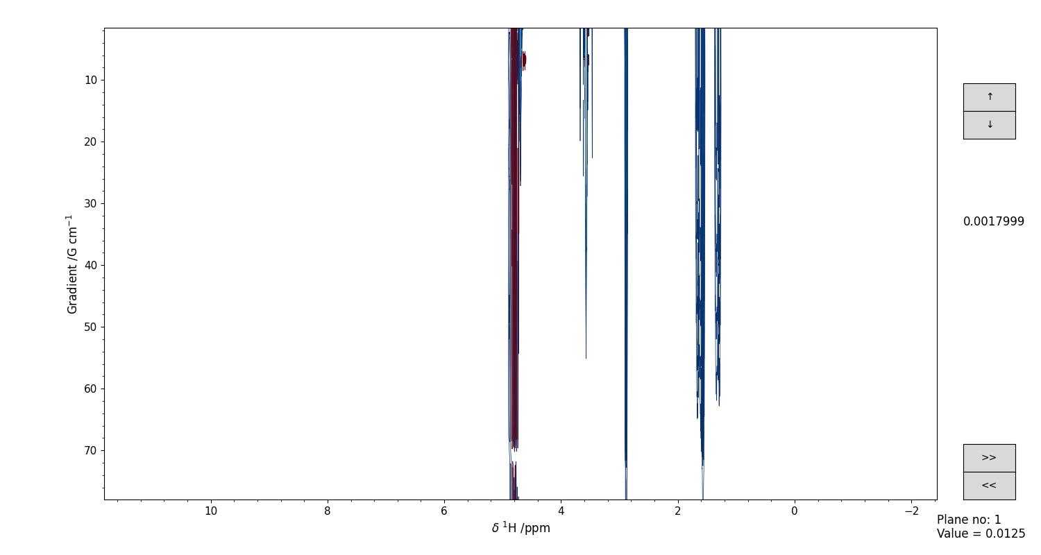
Figure 8 GUI for the interactive visual inspection of a DOSY-T1 spectrum. Use the “>>” and “<<” buttons to move across the planes, and the mouse scroll to move the contour levels.
Analyzing data in KLASSEZ
Evaluate Signal to Noise Ratio
In KLASSEZ, the signal to noise ratio (SNR) of a spectrum is defined as the height of the tallest peak
(or of the reference peak, chosen by the user) divided by twice the standard deviation of the noise.
To estimate the SNR of a 1D spectrum, the function klassez.anal.snr() is used:
s = kz.Spectrum_1D(path/to/dataset)

# ...

s_reg = (5, 4)
n_reg = (0, -2)

snr = kz.anal.snr(s.ppm, s.r, s_reg=s_reg, n_reg=n_reg)
The user has to specify the region where to find the reference signal (s_reg) and a signal-free region (n_reg)
for the evaluation of the noise standard deviation.
It is also possible to set them interactively by using a dedicated GUI:
snr = kz.anal.snr(s.ppm, s.r, gui=True)
which appears like in Figure 9. Here, the regions of signal and noise are highlighted with colored span selectors. There is also a display of the noise level, via two dashed red lines. If these lines do not visually match with the noise, most likely the user has included a signal within the noise region.
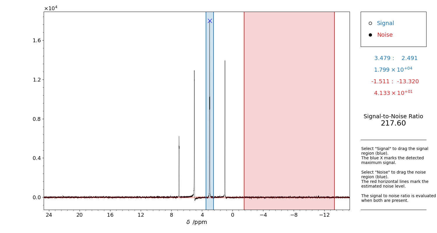
Figure 9 GUI for the evaluation of the Signal to Noise Ratio of a 1D spectrum.
Select “Signal” on the top right corner and drag a region to highlight the reference signal approximate position. The detected point appears as a blue X.
Then, select “Noise”. Drag a signal-free region, i.e. where there is only noise. This will be used for the estimation of the noise standard deviation. The noise level will be highlighted in the figure by two red dashed lines. If these lines do not visually match the noise level, it is most likely there is a signal included in the noise region.
When both the signal and the noise are present, the SNR will be computed.
The selection can be refined as many times as one wants, until the figure panel is closed.
Close the figure to return the values, and to print the used s_reg and n_reg to be given
to klassez.anal.snr().
The procedure for estimating the SNR of a 2D spectrum is equivalent to the 1D case.
s = kz.Spectrum_2D(path/to/dataset)

# ...

s_reg = [(5, 4), (114, 110)]
n_reg = (-2, 102)

snr_f1, snr_f2 = kz.anal.snr_2D(s.ppm_f1, s.ppm_f2, s.rr, s_reg=s_reg, n_reg=n_reg)
In this case, s_reg delimits a rectangular region where to search for the highest signal. In the example above,
the instruction says the reference signal is between 5 and 4 ppm in the direct dimension and between 114 and 110 ppm in the indirect dimension.
As the definition of what the SNR of a 2D spectrum actually is is quite ambiguous, KLASSEZ estimates the SNR for the direct and indirect dimension
independently. This is the reason why the function returns two values.
The estimate of the noise standard deviation is performed on two signal-free traces, extracted on the indirect and the direct dimension, where indicated by n_reg.
In this example, n_reg = (-2, 102) means the noise-only trace of the indirect dimension must be taken at -2 ppm in the direct dimension chemical shift scale, and the one of the direct dimension must be taken at 102 ppm of the indirect dimension.
Also in this 2D case it is possible to use a GUI:
snr_f1, snr_f2 = kz.anal.snr(s.ppm_f1, s.ppm_f2, s.rr, gui=True)
which appears like in Figure 10. The region where to search for the reference signal is drawn with a rectangle selector. The noise-only traces are extracted using a crossmark-like cursor.
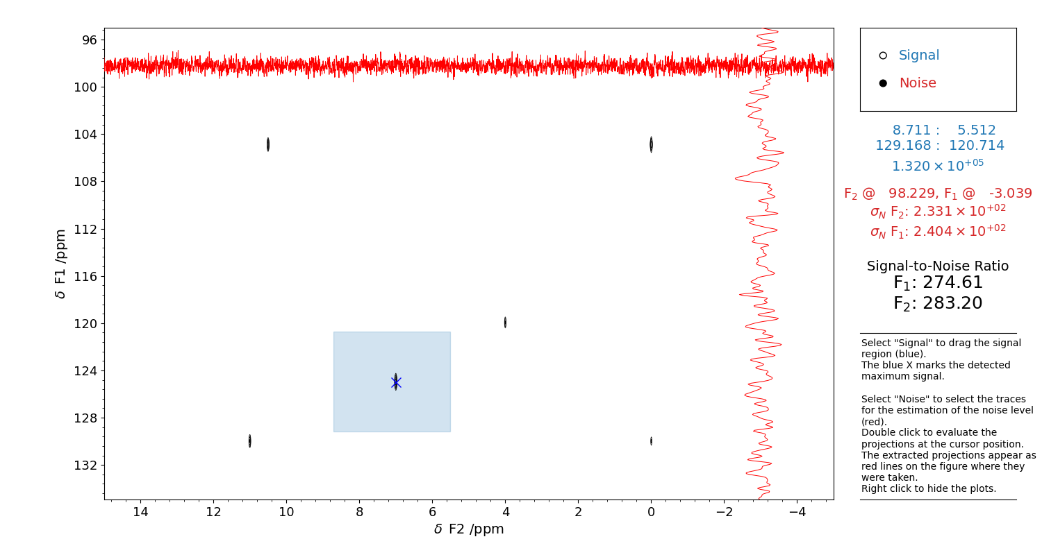
Figure 10 GUI for the evaluation of the Signal to Noise Ratio of a 2D spectrum.
Select “Signal” on the top right corner and drag a rectangle to highlight the reference signal height. The detected point appears as a blue X.
Then, select “Noise”. A red cross-cursor will appear. Find a position where you can extract a signal-free region, i.e. where there is only noise. Double click with the left button of the mouse to extract the projection in that point: they will appear as red traces. These will be used for the estimation of the noise standard deviation.
When both the signal and the noise are present, the SNR will be computed.
The selection can be refined as many times as one wants, until the figure panel is closed.
Close the figure to return the values, and to print the used s_reg and n_reg to be given
to klassez.anal.snr_2D().
Integrate 1D spectra
A 1D spectrum represented by the class klassez.Spectra.Spectrum_1D can be interactively integrated with a dedicated GUI, that calls for klassez.anal.integrate(), by typing:
s.integrate()
An example of such interface is shown in Figure 11.
The integrals are computed according to the fundamental theorem of calculus (see klassez.processing.integrate()), using the frequency (Hz) scale as independent variable.
The obtained values are normalized to the FID intensity. In NMR, the intensity (i.e. the integral) of the whole spectrum
is given by the first point of the FID. To preserve this information (which is something that klassez indeed does), it is required to
apply a conversion factor to the “raw” integrals equal to twice the dwell time (2 * self.acqus['dw']).
The self.integrals attribute is a dictionary that has the strings {ppm1:.3f}:{ppm2:.3f} as keys, with ppm1 and ppm2 being the
ppm values that delimit the integration regions. Each key is associated with the integral of that region.
It is also possible to integrate the spectrum “blindly”, i.e. without using the GUI, by specifying the integration regions. The limits must be passed to the function as a list of 2-entry-tuples, the latter containing the integration regions:
lims = [[3, 2], [9, 8]]
s.integrate(lims=lims)
If you have a given spectrum t that you already integrated, and you want to integrate the spectrum s on the same regions, you can easily convert
the keys of t.integrals to the limits by using the function klassez.misc.key_to_limits():
limits = misc.key_to_limits(list(t.integrals.keys()))
s.integrate(lims=limits)
After each call of the integrate() function, a section of a <filename>.igrl file is written.
Such file can be loaded by calling the klassez.Spectra.Spectrum_1D.read_integrals() method with the name of the file to read:
s.read_integrals(filename='myfilename.igrl')
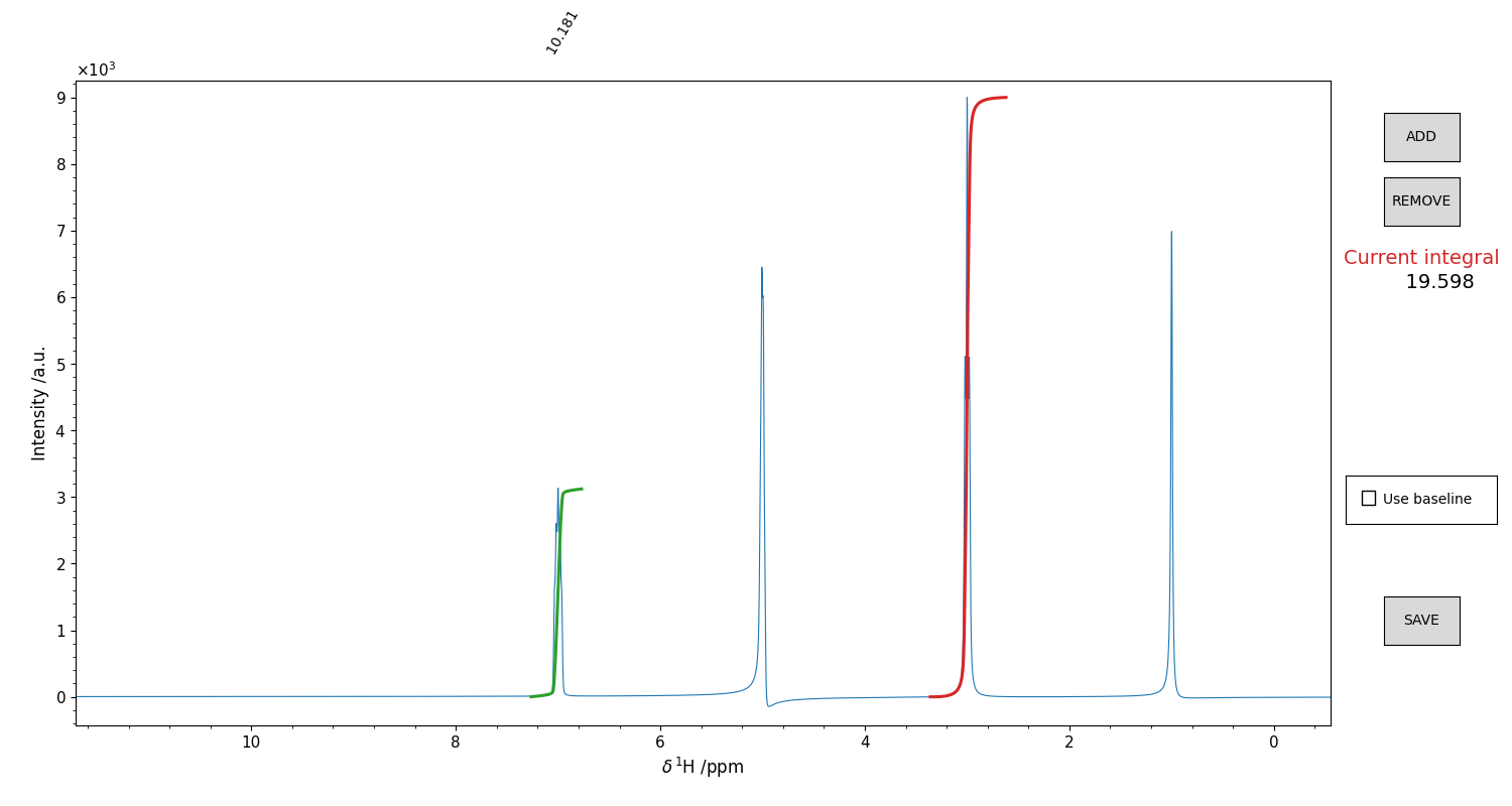
Figure 11 GUI for the integration of 1D spectra. Drag and drop the mouse to highlight an integration region. The integral will appear as a red trace on top of the spectrum. The height is not indicative of the value (which is written on the right), but it is not important, as it is the shape of that curve that matters. It is possible to include a “baseline” for the calculation, that is basically the straight line that connects the borders of the integration window. Might be useful sometimes. Once you are satisfied with the integral, press the ADD button. The integral function plot from red becomes green, and you can integrate another region. Repeat this procedure for as many peaks as you want. To remove an integral from the list, click on the correspondant integral value displayed in black above the top border of the figure. The integral should become blue. Press “REMOVE” to remove it. Once you integrated all the regions you were interested in, press “SAVE” to close the figure and write the .igrl file.
Deconvolution of 1D datasets
The class klassez.fit.Voigt_Fit in KLASSEZ offers a very convenient
interface to deconvolve a spectrum by fitting. A shortcut to the class,
which initializes the parameters automatically, is instanced in the
attribute F of Spectrum_1D.
Creating an initial guess for the fit
To generate the input guess for the fit, you have to call the method
iguess() of the class. This can work in two different modes: the
default one, which allows to build the guess peak-by-peak (Figure 12), and with
auto=True, that features a peak-picker for the selection (Figure 13). The former
is more precise, the second is much faster.
The “manual” mode allows to optimize a polynomial baseline for each interval. A button labelled “SET BASL” must be pressed when a satisfying region is highlighted in the GUI: this allows the scale on which the baseline is computed to be correctly aligned to the region itself. When this step is correctly performed, the box next to the button turns from red to green. Should the region be moved during the optimization of the initial guess, the box turns back to red, and the “SET BASL” button must be pressed again to adjust the baseline scale accordingly.
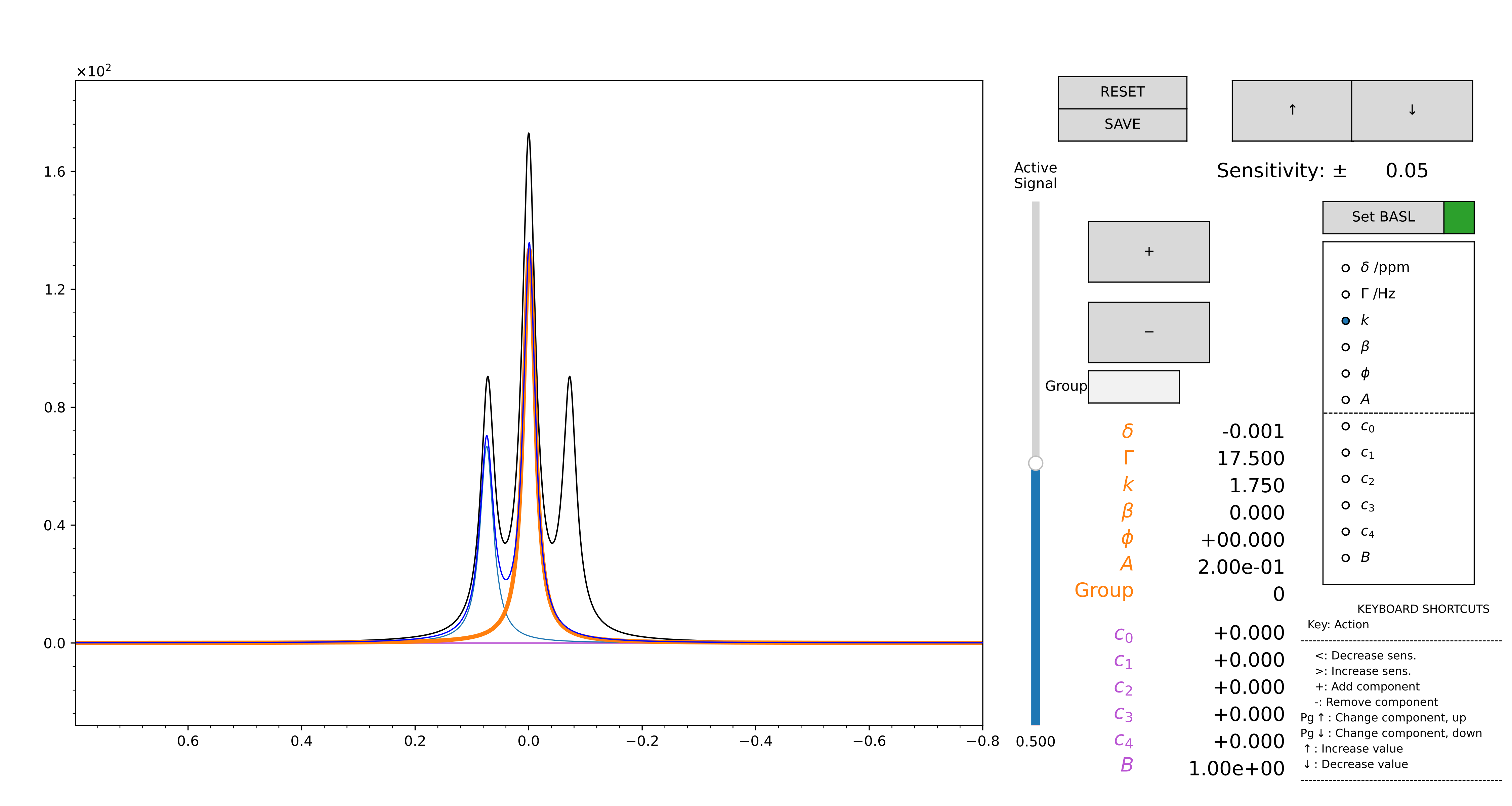
Figure 12 GUI for the computation of the initial guess, in manual mode. Zoom on the region you want to model using the lens. Then, press “SET BASL”: the red square icon should become green. This allows to set the limits for the baseline.
At this point, use the “+” button to add a component. You can select the parameter of the selected component to change by selecting it in the radiobuttons on the right: chemical shift, linewidth, relative intensity, phase, fraction of gaussianity. The mouse scroll controls the variation of the active parameter. The parameter “A” changes the intensity of all the components together. The parameters “c0”, “c1”… are the coefficient of a 4th order polynomion. “B” is an intensity factor that multiplies all the “c”s.
Use the slider to change the active component. The arrow buttons at the top control the sensitivity of the mouse scroll.
When you are satisfied with the model, press “SAVE”. The original zoom is restored, and the modelled region appears highlighted in green. Repeat the process as many times as you want. The .vf file is written every time the “SAVE” button is pressed. When you are done, just close the figure.
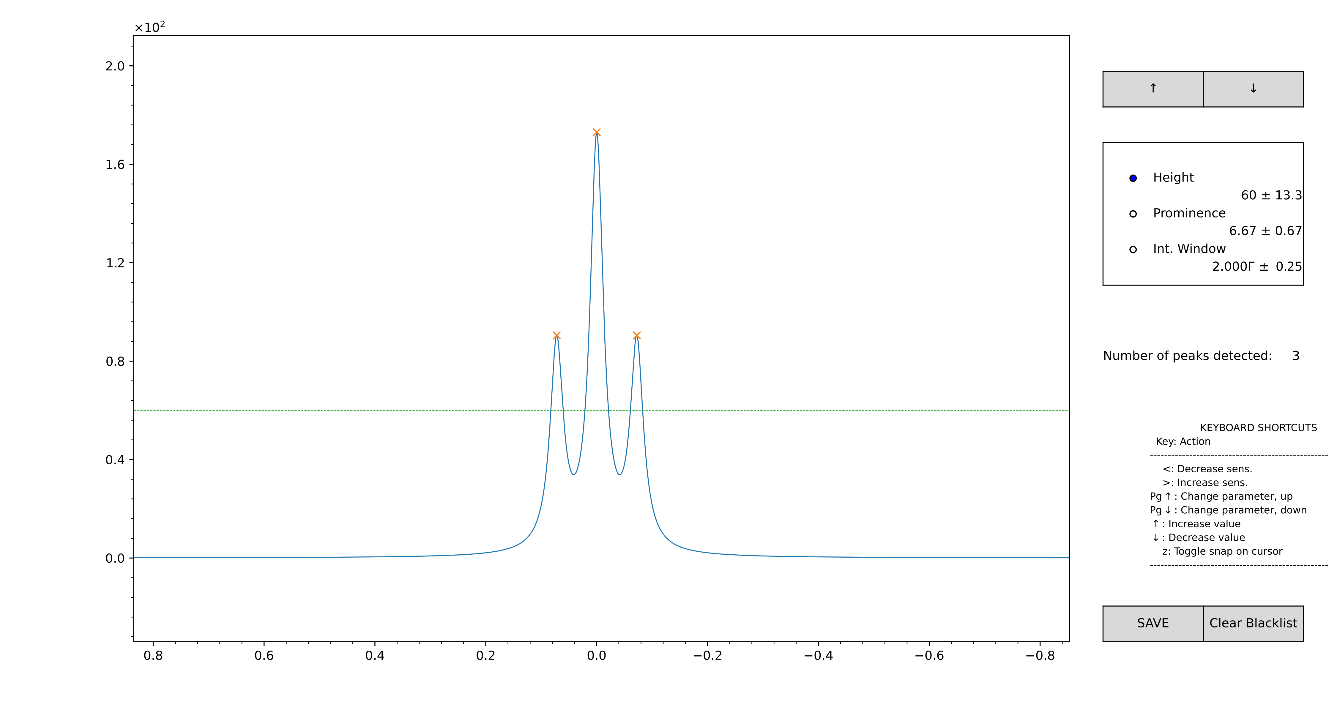
Figure 13 GUI for the computation of the initial guess, in automatic mode. Zoom on the region you want to model using the lens.
At this point, use the scroll of the mouse to adjust the height and the prominence for the peak-picker. The integration window, used to estimate the intensity of the components, can be adjusted as well. The detected positions are marked with a “x”. If you want to add a peak that is not included automatically, double-click on the interested position: these will appear with a “+”. If you want to remove an automatically detected position, right-click.
When you are satisfied with the model, press “SAVE”. The original zoom is restored, and the modelled region appears highlighted in green. Repeat the process as many times as you want. The .vf file is written every time the “SAVE” button is pressed. When you are done, just close the figure.
The .vf files
The information on the peaks is saved in a .vf file, which can be
imported with the function klassez.fit.read_vf`(). There are two kind of
.vf file: .ivf, that marks initial guesses, and .fvf, for
the results of the fit. However, this is a human-only distinction, as
the structure of the files is the same.
An example of .vf file is shown here:
! Initial guess computed by francesco on 11/11/2024 at 15:48:44

          Region;      Intensity
------------------------------------------------------------------------------------------------
 193.317:168.041;   8.08246575e+00

   #;              u;           fwhm;    Rel. I.;      Phase;       Beta;      Group
------------------------------------------------------------------------------------------------
   1;   179.94060191;     172.500000;   1.000000;    -10.000;    0.00000;          0
------------------------------------------------------------------------------------------------

================================================================================================

          Region;      Intensity
------------------------------------------------------------------------------------------------
    59.936:6.662;   5.02908980e+01

   #;              u;           fwhm;    Rel. I.;      Phase;       Beta;      Group
------------------------------------------------------------------------------------------------
   2;    40.29851786;     150.000000;   0.214286;      0.000;    0.00000;          0
   3;    24.98695246;     140.000000;   0.785714;     10.000;    0.00000;          0
------------------------------------------------------------------------------------------------

================================================================================================
The header line, that starts with a !, is a comment, and acts as a
separator between different attempts of the fit. In fact, .vf files
are never overwritten: working again on the same file appends the
information at the bottom. Hence, there is a parameter n in the
klassez.fit.read_vf() function that allows to select which attempt to read.
Then, a series of blocks follow. Each block marks a region of selection: the keys “Region” and “Intensity” mark the limits of the fitting window, and the total intensity of the peaks. Under this line, there is a table that collects the peak parameters. As a final information there might be the baseline coefficients for the given region, which start with the key “BASL_C”. Should this line be missing, it means that the baseline was not optimized during the computation of the guess, and the coefficients will all be set to 0 when the file is read. The end of the block is marked with a line of “=”.
The method iguess() automatically search for the existing input file.
If it finds it, it is automatically loaded. Otherwise, the GUI for the
computation of the initial guess opens up.
Editing the initial guess via GUI
After having loaded the initial guess (and therefore having it stored in the i_guess
attribute), it is possible to modify it interactively using a dedicated GUI.
To do so, you have to call the method edit_iguess(), which is an indirect call
for the function klassez.gui.edit_vf() (Figure 14).
Example:
# ``s`` is a ``Spectrum_1D`` object
s.F.iguess(filename='test', ext='ivf')       # reads 'test.ivf'
s.F.edit_iguess(filename='test', ext='ivf')  # editing adds and extra section in the same file
In this interface, the initial guess is loaded as a total trace in blue, and the experimental spectrum in black.
In order to minimize the rendering time, the GUI is initialized in “locked” state, which means that all the peaks cannot be edited right-away, and are therefore static traces. Double-click with the left button of the mouse on a region to select it: from green it will become violet. To change the limits of the region, press the “Change Window Limits” button. The highlighted region will become red, and you can drag it to adjust the position of the window limits. Press the button again to store the new values.
To edit the model of a region, after you selected it, press the “UNLOCK” button. The peaks that contribute to that region gets unpacked, and become editable (“unlocked” state of the GUI). Use the slider to move between the various components, and the mouse scroll to change the model parameters. Use the “+” and “-” buttons to add or remove components. Press “LOCK” to save your modification. Press “RESET” to restore the region model as it was before pressing “UNLOCK”. Both these actions bring the GUI back to “locked” state.
To add a new region, select the region of the spectrum you want to fit by focusing the zoom on it using the lens button. Then, press the “New Region” button, that will become yellow, and the GUI passes in “unlocked” state with no initialized peaks there. Add and move the components as you would do to edit a pre-existing region. Press “LOCK” to save the new region.
To remove a region, UNLOCK it and remove all the components, then press “LOCK”. The associated green span will disappear.
At the end, press “SAVE and EXIT” to write the edited .vf file and close the GUI.
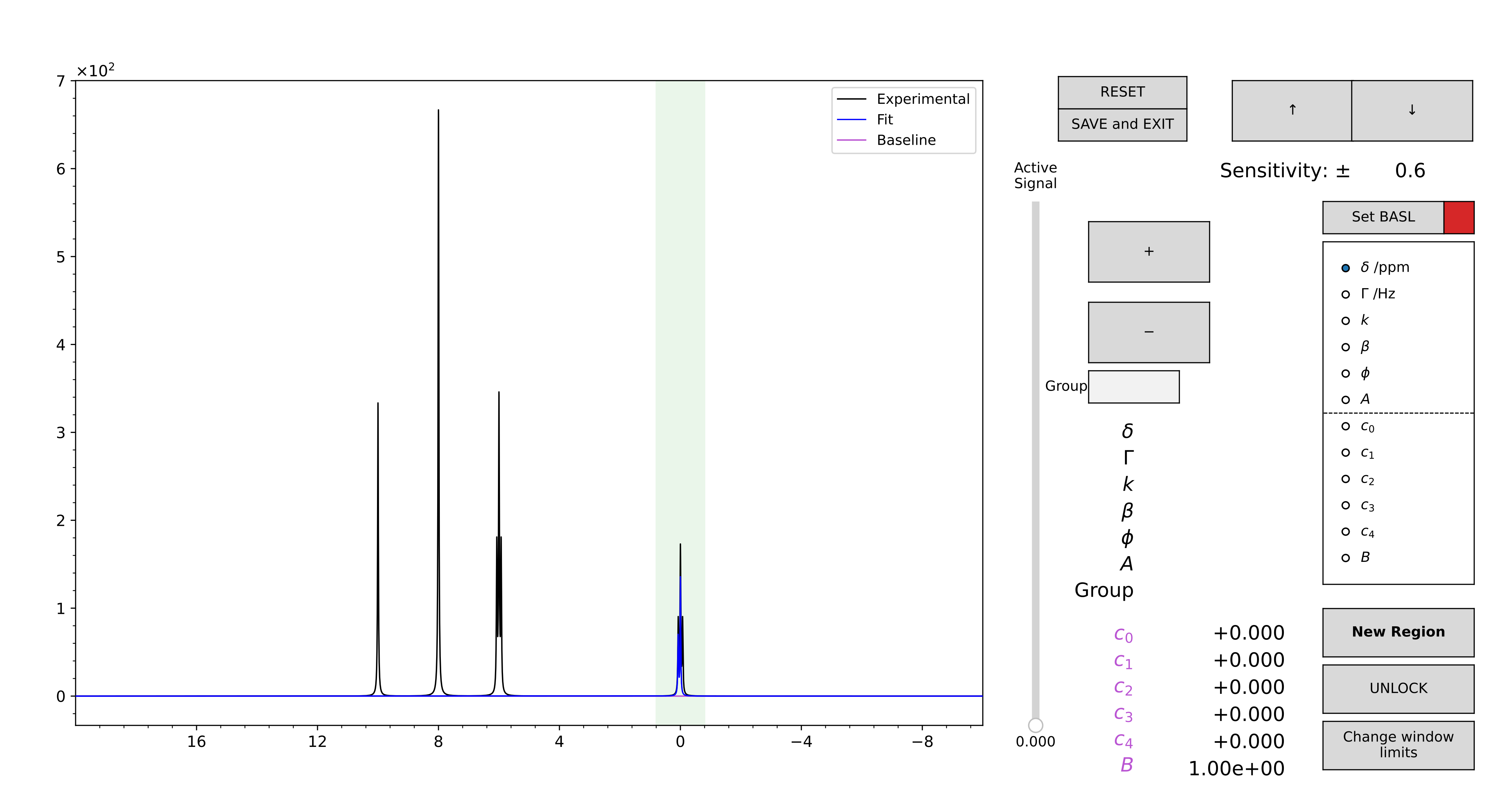
Figure 14 GUI for the editing of a guess, read by a .vf file.
The usage is thoroughly described here or in the documentation of the klassez.gui.edit_vf() function.
Doing the fit
The fit can be performed by calling the method klassez.fit.Voigt_Fit.dofit(), which returns
a list of lmfit.MinimizerResult objects (one for each region) for a
detailed inspection on how the fit performed. The behavior of the fit
can be customized by setting the parameters of the method (see examples
or the dedicated page of the manual).
Generally speaking, the method can be called as
filename = 'output'
s.F.dofit(filename=filename,        # writes 'output.fvf'
          method='leastsq',
          itermax=10000,
          fit_tol=1e-08,
          u_lim=1,                  # ppm
          f_lim=10,                 # Hz
          k_lim=(0, 3),
          ph_lim=(-180, 180)        # degrees
          vary_phase=False,
          vary_b=True,
          basl_fit='no',
          )
We recommend to use method='leastsq', as for this kind of optimization is the best compromise
between speed and accuracy. It is also possible to run multiple optimization in sequence by specifying
multiple methods in a list, e.g. method=['leastsq', 'leastsq'].
Should the fit be very complicated, the maximum number of iteration can be increased (or decreased) by changing
the itermax parameter.
The selectivity of the arrest criterion can be tuned through fit_tol.
The tolerances for the various peak parameters are very important for the correct outcome of the fit.
u_lim controls the limits of the chemical shift for each component: if the initial guess for the chemical
shift is u, then this value during the fit can vary between u - u_lim and u + u_lim ppm.
No matter what, the chemical shift cannot fall out of the window!
More critical is the choice of the limits for the linewidths, through f_lim, which is in Hz (thus more sensitive).
The linewidth of each component can vary from the initial guess of +/- f_lim. The minimum linewidth possible is 0 Hz.
The intensity limits are controlled by k_tol, which can be either one or two values.
If it is a single value, the relative intensity of each component can vary of +/- k_tol with respect to the initial guess.
If it is a sequence of two values, the relative intensity can vary between min(k_tol) and max(k_tol).
About ph_lim, it is quite intuitive. Normally, you fit a phased spectrum, hence you will have to set vary_phase=False
to decrease the computational cost of the fit. However, if you want to optimize also the phases of the peaks, these limits are very important
to be set especially if you have a dataset that features both positive and negative peaks, as there is the possibility that the fit
will try to match a negative peak with a 180° phase.
vary_b allows to change the fraction of gaussianity of each component during the fit, ranging from 0 (pure Lorentzian) to 1 (pure Gaussian).
basl_fit controls the fit of the baseline:
basl_fit="no": Do not use baseline (default)
basl_fit="fixed": The baseline is computed once and kept fixed during the optimization
basl_fit="fit": The baseline coefficients enter as fit parameters during the nonlinear optimization
basl_fit="calc": The baseline coefficients are calculated during the optimization via linear least-squares optimization
The fit goes region-by-region, and the results are saved in a .fvf file.
A .fvf file can be loaded using the method load_fit().
Once loaded, it is possible to edit also that via GUI by calling the edit_result()
method, which works exactly the same as editing an initial guess.
Plot results
Either the initial guess or the result of the fit can be conveniently
visualized by using the method plot(). Alternatively, the arrays of
the model can be retrieved by calling calc_fit_lines(). The method
res_histogram() computes the histogram of the residuals, for a better
understanding of the outcome of the fit procedure.
Vide infra for a working example.
Integrate a pseudo-2D spectrum
The method klassez.Spectra.Pseudo_2D.integrate() differs a little bit from the one coded in
Spectrum_1D, but essentially from the user’s perspective it works the same.
s.integrate(ref=0)
The GUI (Figure 15) will display all the transient stacked one to each other. The integral function
that will appear when dragging the region refers to the reference spectrum, whose index is passed through the ref argument, but in the
side panel on the bottom left it will appear how the trend of the integrals throughout
the whole series will look like.
When pressing SAVE, the integrals will be saved in a .igrl file, as in the 1D case,
to be recovered with the method klassez.Spectra.Pseudo_2D.read_integrals().
s.read_integrals(filename='myfilename.igrl')
The self.integrals attribute is a dictionary that has the strings {ppm1:.3f}:{ppm2:.3f} as keys, with ppm1 and ppm2 being the
ppm values that delimit the integration regions. Each key is associated with the integrals of that region throughout the series, as 1darray.
As in the 1D case, it is possible to integrate the spectrum “blindly”, i.e. without using the GUI, by specifying the integration regions. The limits must be passed to the function as a list of 2-entry-tuples, the latter containing the integration regions:
lims = [[3, 2], [9, 8]]
s.integrate(lims=lims)
If you have a given spectrum t that you already integrated, and you want to integrate the spectrum s on the same regions, you can easily convert
the keys of t.integrals to the limits by using the function klassez.misc.key_to_limits():
limits = misc.key_to_limits(list(t.integrals.keys()))
s.integrate(lims=limits)
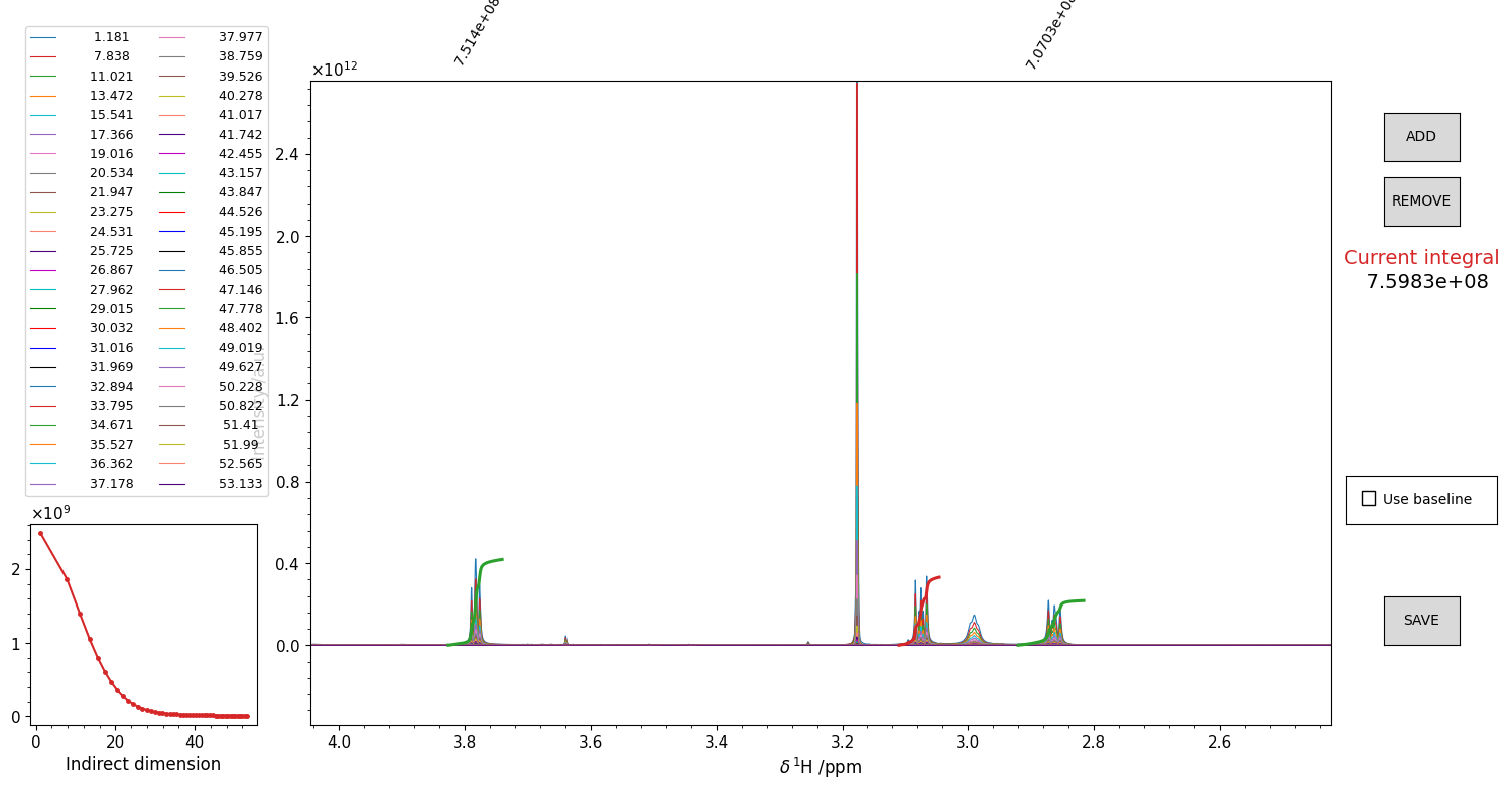
Figure 15 GUI for the integration of pseudo-2D spectra. Drag and drop the mouse to highlight an integration region. The integral of the reference spectrum will appear as a red trace on top of the spectrum. The height is not indicative of the value (which is written on the right), but it is not important, as it is the shape of that curve that matters. It is possible to include a “baseline” for the calculation, that is basically the straight line that connects the borders of the integration window. Might be useful sometimes. The trend of the computed integrals throughout the series appears in the side panel. Once you are satisfied with the integral, press the ADD button. The integral function plot from red becomes green, and you can integrate another region. Repeat this procedure for as many peaks as you want. To remove an integral from the list, click on the correspondant integral value displayed in black above the top border of the figure. The integral should become blue. Press “REMOVE” to remove it. Once you integrated all the regions you were interested in, press “SAVE” to close the figure and write the .igrl file.
Fitting a DOSY
In the present release, klassez.fit.DosyFit supports the fit for single and double stimulated echoes, with or without bipolar gradients
(sequences ste, stebp, dste, dstebp).
The important attributes of the klassez.fit.DosyFit class are:
self.g: 1darray that contains the difflist converted to Tesla / meter (so that the diffusion coefficient comes in \(m^2 s^{-1}\);self.data: dictionary that contains the integrated values of the parent spectrum using the integration region as a key formatted as{ppm1:.3f}:{ppm2:.3f};self.dosy_par: dictionary of the parameters that will be employed by the model during the fit.
# Fit of the DOSY
#   Make/read initial guess
s.D.iguess(filename=filename)
#   Fit the data
s.D.dofit(filename=filename)
#   Plot the fits
s.D.plot(filename=filename, dpi=200)
#   Make a figure of the diffusion coefficients
s.diffplot(filename=filename, dpi=200)
The method klassez.fit.DosyFit.iguess() allows to generate an oculated initial guess for all the integrated regions.
More than one component can be used at once for a single region. The user can adjust the relative fraction of the various components,
as well as to adjust the intensity factor automatically or not. Example and additional explanation in Figure 16.
Computing the initial guess creates a file <filename>.idy, that can be read with klassez.fit.read_dy().
If the file already exists, it will be loaded and stored in the attribute self.i_guess.
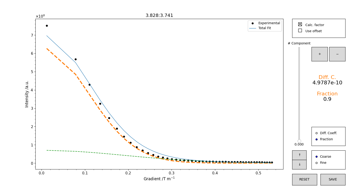
Figure 16 GUI for the initialization of the diffusion coefficient. The integrals trend will appear as black points. The total model is the blue trace. Use the mouse scroll to change either the value of the diffusion coefficient or the fraction, according to the selector on the right part of the figure. It is possible to change the sensitivity of the scroll with the selector “coarse/fine”, or with the arrow buttons. Use the “+” button to add a component. Use the vertical slider to change component to edit. The check button at the top toggles the computation of the intensity factor. Deactivate it to gain more freedom in adjusting the relative fraction when trying to adjust multiple components. DO NOT INCLUDE the offset unless you have a very specific reason to do so. When you are satisfied with your guess, press “SAVE” to save it.
At this point, the fit can be performed by calling the method klassez.fit.DosyFit.dofit().
A number of parameters for the fit can be adjusted. The model function is selected automatically on the basis
of the employed pulse sequence (see klassez.fit.DosyFit.select_model()).
The results of the fit will be saved in a file named <filename>.fdy. A new entry of the file will be added at the bottom.
This file will never be overwritten automatically by the program.
Alternatively, the results of a previously performed fit can be read from a .fdy file by the method klassez.fit.DosyFit.load_fit().
In both cases, the outcome will be stored in the attribute self.result.
Now it is the time to see how the fit looks like.
The klassez.fit.DosyFit.plot() method generates the figure of the fitted trends, that also display the diffusion coefficient value in the legend.
A number of parameters for the figure can be tuned, such as dimension, resolution and format of the figure to save, to display the residuals or not, etc.
When the fit is either performed or loaded (i.e. the attribute self.D.result exists), the parent DOSY object gains access to the klassez.Spectra.DOSY.diffplot().
This function will generate a figure that display an upper panel with the whole spectrum, and a bottom panel with the fitted diffusion coefficients.
The integrated regions will be highlighted as light-blue spans in both panels. This will be useful to compare the different diffusion coefficients associated to the various regions, and therefore to the chemical species present in the sample.
Fitting a DOSY-T1
Conceptually, the fitting of a klassez.Spectra.DOSY_T1 is equivalent to fitting a series of DOSY spectra, as described in the previous section.
However, there exist the class klassez.fit.Fit_Dosy_pp3D to make it easier.
The first thing to do is to integrate the dataset, that can be easily done with
s.integrate(filename='custom_filename') # or None for the default
This command will create an instance of the klassez.fit.Fit_Dosy_pp3D class, and will store it in the attribute D of the klassez.Spectra.DOSY_T1 object.
In practice, from now on we can proceed with the fit by calling the methods as s.D.method().
The reason why this method is called integrate and not instance_D or similar is because klassez.fit.Fit_Dosy_pp3D.__init__() will either compute or read the integrals of all the planes of the spectrum.
The function will try to find the .igrl files in a folder named <filename>. If it does not find them, it will open the GUI of Figure 15 to integrate
interactively the first plane of the series. The same regions will be used to integrate all the others, and the aforementioned .igrl files are written automatically.
This means that at the second call of s.integrate(), there will be no need of computing the integrals again.
At this point you have to create the initial guess for the diffusion coefficient for each of the integrated region.
s.D.iguess(filename='custom filename') # if you want
As explained in the DOSY section, it is not required to have a super-accurate initial guess, the important thing is to have the correct number of components that you want to include in the fit. The GUI is the same of Figure 16. This function will write the .idy files required for starting the fit.
Now you can fit the data with
s.D.dofit(seq=False, filename='custom filename') # now you know the drill
The important point to remember here is that the default behavior of this function is to use the same diffusion coefficient to fit the same region across all planes.
This aspect will improve the robustness of the results.
If you do not want this, and you want to fit each plane with its diffusion coefficient, run the function with seq=False.
At the end of the fit, a series of .fdy files are written.
These can be read by
s.D.load_fit(filename='custom filename')
To visualize the results of the fit, the method klassez.fit.Fit_Dosy_pp3D.plot() will generate the figure for you.
The function has a lot of parameters:
s.D.plot(what='result',         # or 'iguess'
         only_all=False,        # Save only the comprehensive figure
         show_res=False,        # For the single plots
         res_offset=0,          # For the single plots
         figdir=None,           # Default (None) or custom figure directory
         filename=filename,     # Root filename for the figures
         ext='svg',             # Figure format
         dpi=100,               # Resolution in dots per inches
         dim=None               # Default (None) or custom figure size (inches)
         )
Set what to either 'iguess' or 'result' to plot the initial guess or the fit results, respectively.
All the figures will be saved in figdir/what, with a name that starts with filename and the interval.
The parameter only_all, if set to True, will generate only a set of comprehensive figures where the profiles and their fit for all planes are plotted
together in the same panel. If it is False, also one figure per interval per plane are saved. This might take a lot of time, hence it is recommended to turn this to False at the very end of the fitting trials (and if you really need these very detailed figures).
Example scripts
Reading and processing of 1D spectra
#! /usr/bin/env python3

from klassez import *

# Be aware that this is a BASIC processing
# Read the documentation of the functions to see the full powers

if 1:
    # This example is for the simulated data
    s = Spectrum_1D('acqus_1D', isexp=False)
    # You can convert info on peaks to .ivf for fitting
    s.to_vf()
else:
    # Use the following to read experimentals:
    spect = 'bruker', 'jeol', 'varian', 'magritek', 'oxford' # One of these
    s = Spectrum_1D(path_to_dataset, spect=spect)
# Setup the processing
#   Apodization
#   Follow the table in the user manual to see what reads what
s.procs['wf']['mode'] = 'em'
s.procs['wf']['lb'] = 5
#   Zero-filling
s.procs['zf'] = 2**14
#   Apply processing and do FT
s.process()
#   Remove the digital filter
s.pknl()

#   Phase correction
s.adjph()

#   Calibration
s.cal(from_procs=False)

#   Remove solvent
s.qfil(from_procs=False)

# Plot the data
s.plot()

# Integrate the spectrum
s.integrate()
Fit 1D spectrum
The beginning of the script is the same of the reading example.
# s.F is a fit.Voigt_Fit object
filename = 'test_1D_fit'    # base filename for everything fit-related
# Compute the initial guess
auto = False        # True for peak-picker, False for manual
s.F.iguess(filename=filename, auto=auto)

if 0:   # Do the fit
    lmfit_result = s.F.dofit(   ### Parameters of the fitting ###
            u_lim=5,            # movement for chemical shift /ppm
            f_lim=50,           # movement for linewidth /Hz
            k_lim=(0, 3),       # limits for intensity
            vary_phase=True,    # optimize the phase of the peak
            vary_b=True,        # optimize the lineshape (L/G ratio)
            method='leastsq',   # optimization method
            itermax=10000,      # max. number of iterations
            fit_tol=1e-10,      # arrest criterion threshold (see lmfit for details)
        basl_fit='fixed'    # how to handle the baseline during the fit
            filename=filename,  # filename for the .fvf file
            )
else:
    # Load an existing .fvf file
    s.F.load_fit(filename=filename)

# Plot the results
s.F.plot(what='result',     # what='iguess' for initial guess
         show_total=True,   # Show the total trace or not
         show_res=True,     # Show the residuals
         res_offset=0.1,    # Displacement of the residuals (plots residuals - res_offset)
         labels=None,       # Labels for the peaks
         filename=filename, # Filename for the figures
         ext='png',         # format of the figure
         dpi=300,           # Resolution of the figure
         )

# Compute histogram of the residuals
s.F.res_histogram(what='result',
              nbins=500,    # Number of bins of the histogram
              density=True, # Normalize them
              f_lims=None,  # Limits for x axis
              xlabel='Residuals',   # Guess what!
              x_symm=True,  # Symmetrize the x-scale
              barcolor='tab:green',     # Color of the bars
              fontsize=20,  # Guess what!
              filename=filename, ext='png', dpi=300)

# Convert the tables of numbers in arrays
peaks, total, limits, whole_basl = s.F.get_fit_lines(what='result')
Read and process 2D spectrum
 #! /usr/bin/env python3

 from klassez import *

 # Be aware that this is a BASIC processing
 # Read the documentation of the functions to see the full powers
 if 1:
     # This example is for the simulated data
     s = Spectrum_2D('acqus_2D', isexp=False)
 else:
     # For experimentals, at version 0.4a.7 klassez reads only 2D bruker
     s = Spectrum_2D(path_to_dataset)

 # Setup the processing
 #   Apodization
 #   Follow the table in the user manual to see what reads what
 #   REMEMBER: index 0 is F1, index 1 is F2, for procs
 s.procs['wf'][1]['mode'] = 'em'
 s.procs['wf'][1]['lb'] = 5
 s.procs['wf'][0]['mode'] = 'qsin'
 s.procs['wf'][0]['ssb'] = 2
 #   Zero-filling
 s.procs['zf'] = 512, 4096
 #   Apply processing and do FT
 s.process()
 #   Remove the digital filter
 s.pknl()

 #   Phase correction
 s.adjph()

 #   Calibrate
 s.cal()

 #   Remove solvent
 s.qfil()

 # Plot the data
 s.plot()

 # Extract projections
 ppm_f1 = 105
 ppm_f2 = 10
 s.projf1(ppm_f2)
 # Extract F1 trace @ ppm_f2 ppm
 f1 = s.Trf1[f'{ppm_f2:.2f}']
 # Call it back: it is a Spectrum_1D object!
 f1.plot()
 s.projf2(ppm_f1)
 # Extract F2 trace @ ppm_f1 ppm
 f2 = s.Trf2[f'{ppm_f1:.2f}']
 # Call it back: it is a Spectrum_1D object!
 f2.plot()
Read and process a pseudo-2D and fit DOSY
Pseudo_2D is the same! #! /usr/bin/env python3
from klassez import *
# Read the spectrum
s = DOSY('path/to/dataset/expno')
# Processing
# Window function: exponential with 0.5 Hz linebroadening
s.procs['wf']['mode'] = 'em'
s.procs['wf']['lb'] = 0.5
# Zerofill to twice the size
s.procs['zf'] = 2 * s.fid.shape[-1]
# Apply and do FT
s.process()
# Remove digital filter
s.pknl()
# Phase the spectrum (uncomment to do it!)
s.adjph()
# Plot the spectrum to see it
s.plot_md()
# Analysis
filename = 'test'
# Integrals
if 1: # compute the integrals
s.integrate(filename=filename)
else: # read an integrals file
s.read_integrals(filename=f'{filename}.igrl')
# Fit of the DOSY
# Make/read initial guess
s.D.iguess(filename=filename)
# Fit the data
s.D.dofit(filename=filename)
# Plot the fits
s.D.plot(filename=filename, dpi=200)
# Make a figure of the diffusion coefficients
s.diffplot(filename=filename, dpi=200)
Read, process and fit a DOSY-T1
 #! /usr/bin/env python3

 import klassez as kz

 # Path to dataset
 path = 'path/to/dataset/expno'
 # Read the dataset
 s = kz.DOSY_T1(path)

 # Usual processing
 s.procs['wf']['mode'] = 'qsin'
 s.procs['zf'] = s.fid.shape[-1] * 2
 s.process()
 s.pknl()    # remove group delay

 # Adjust the phase interactively using
 # the ``expno``-th spectrum taken from
 # plane ``fromplane`` in the direction
 # ``dim`` as reference
 s.adjph(fromplane=0, expno=0, dim='31')

 # Plot interactively all the planes F3-F1
 s.plot(dim='31')
 # Plot interactively all the planes F3-F2
 s.plot(dim='32')

 # Extract all the plane in the F3-F1 direction
 if 0:
     P31 = [s.getplane(x) for x, _ in enumerate(s.x_f2)]
     #   Plot all of them
     for q in P31:
         q.plot()
     # Extract all the plane in the F3-F1 direction
     P32 = [s.getplane(x, '23') for x, _ in enumerate(s.x_f1)]
     #   Plot all of them
     for q in P32:
         q.plot()

 # Fitting

 filename = 'My_DOSYT1_spectrum'
 # Integrate the first plane of the F3-F1 direction as reference.
 # If this task was already done, this function will upload the integrals.
 s.integrate(filename=filename)

 # After s.integrate, s.D exists and can be used for fitting
 #   Make initial guess
 s.D.iguess(filename=filename)
 #   Do the fit
 s.D.dofit(filename=filename)
 #   Load the fitted parameters
 s.D.load_fit(filename=filename)
 #   Save the figures
 s.D.plot(what='result',         # or 'iguess'
          only_all=False,        # Save only the comprehensive figure
          show_res=False,        # For the single plots
          res_offset=0,          # For the single plots
          figdir=None,           # Default (None) or custom figure directory
          filename=filename,     # Root filename for the figures
          ext='svg',             # Figure format
          dpi=100,               # Resolution in dots per inches
          dim=None               # Default (None) or custom figure size (inches)
          )
Make figures with KLASSEZ
The module klassez.figures contains a lot of functions that can be used to generate extremely high quality figures, suitable for publications, that can also be made modular.
They work together with a few functions of klassez.misc, responsible for changing fontsizes, appearance of the axes, and so on.
This section of the guide exists to instruct the user on how to create such figures, in order to adapt them to their needs.
The “engine” we will use for computing the figure is based on the matplotlib.pyplot.
We will explain the basics of computing a figure from scratch by using matplotlib’s default functions, hence they might appear redundant to an expert user.
However, we believe it will be useful in particular for non-developers, i.e. people that use, not write, the softwares.
The default figure format employed throughout the whole KLASSEZ package is the Scalable Vector Graphics (.svg).
This choice was made in order to preserve the scalability of the figures without any quality loss, and at the same time keeping the amount of disk space required to the lowest possible amount.
It is of course possible to use bitmap formats: all the figures have the parameter ext, that can be set to whatever figure format the user wants to.
To inspect the pictures, the user must have installed on their computer an image-viewer software.
We recommend the use of eog (“Eye of Gnome”) for linux users, which is lightweight and portable, and has full support for both bitmap and vectorial formats.
On Windows and Mac, where eog is natively not supported, we recommend to use picview (website), that is similar to eog in terms of functionalities.
For further editing of the images (which should not be required in principle, but never say never) we recommend the use of inkscape (website) for vectorials and of GIMP (GNU Image Manipulation Program, website) for bitmap.
As a final remark, please keep in mind that the documentation of matplotlib is one of the most extensive and complete of the entire python environment, and it is also full of examples. Make use of it!
The basics: figure panels and subplots
If a script has to generate a figure at some point, it must of course import the correct module:
import matplotlib.pyplot as plt
We must always start by instantiating a figure panel, i.e. a white canvas that can later host several containers.
It is common practice to keep a hard-reference to it (fig =) in order to be able to edit it later.
fig = plt.figure(figure_title)
figure_title is the string that will appear in the top header of the figure window. If nothing is specified, “Figure 1” will appear.
You can set the dimension of the figure with the command
fig.set_size_inches(width, height)
We recommend to use 15, 8 for visualization plots and 8, 6 for saved figures.
Remember that the fontsizes and thickness of the lines must be tuned accordingly to the dimension of the figure!
The directive
plt.show()
must be used when we want the figure to be rendered and appear on screen. The following example code:
fig = plt.figure('TEST')
fig.set_size_inches(15, 8)

plt.show()
will generate an empty white rectangle, \(15 \times 8\) inches wide, with nothing on it. Very little useful!
In order to make modular figures, and control with very high precision their appearance, we make use of subplots, which are containers for artists (dots, lines, ticks, text, whatever comes to your mind that goes on a figure is an artist).
There are many ways to add subplots to your figure. We will show you two: add_subplot() and add_axes.
The general syntax for add_subplot is
ax = fig.add_subplot(m, n, k)
which essentially means “divide my figure in a grid that has m columns and n rows, number them from 1 to \(mn\), take the number k, and reference it as ax”.
For example, myax = fig.add_subplot(3, 2, 4) will create a grid with three columns and two rows, and myax will be the subplot on the right of the middle row.
Experiment a bit, and read the documentation of matplotlib to explore the full power of this statement!
The subplots positions with respect to fig and to each other can be tuned with the directive
plt.subplots_adjust(left, right, top, bottom, wspace, hspace)
The values associated to these parameter can be taken from the “Configure subplots” button in the interactive figure viewer (which is, with the qtagg framework, the button next to the lens).
add_axes works in a different manner, and for reasons you will clearly understand in a second it is very suitable for insets.
The statement
ax = fig.add_axes([x, y, width, height], transform=transform)
will instantiate as ax a rectangular subplot with the left bottom corner in (x, y), width large and height tall.
As opposed to add_subplot, a subplot created with add_axes is not affected by plt.subplots_adjust in any way.
The numbers we have to write in x, y, width, height depend on the coordinate system we choose, which is declared through the transform parameter.
We need to define two of them. transform=fig.transFigure will use the reference frame of fig, which has the origin in the bottom left corner of the figure panel ((0, 0)) and the top right corner is (1, 1); this will be the one we will use to add “regular” subplots.
For other purposes, we can use the reference frame of another subplot (e.g. ax1) by stating transform=ax1.transAxes. This will instruct the backend to use the values that ax1 has on its axes.
Customizing subplots
In Figure 17 we generated a figure with only one subplot, in order to show which are the main attributes of a subplot and illustrate how to change them.

Figure 17 This is a figure with only one subplot. Each subplot is delimited by four spines and has a title, two axes labels, and certain number of ticks with associated tick labels.
Have you ever seen those very fancy figures of spectra, where there is only the chemical shift scale and the spectrum?
These can be done by setting all the spines invisible except for the bottom one.
This being said, DON’T DO IT. Unless you have a very valid reason to do so.
If such a valid reason exist and you really want to turn the spines off, you can access them via the attribute spines of the subplot itself, which is a dictionary of four elements: 'left', 'right', 'bottom', 'top'.
You can deactivate them with their method set_visible, for example:
ax.spines['left'].set_visible(False)
ax.spines['right'].set_visible(False)
ax.spines['top'].set_visible(False)
Title and axes labels are quite similar in how they can be set:
ax.set_title(new_title)
ax.set_xlabel(new_X_label)
ax.set_ylabel(new_Y_label)
Each of these are matplotlib.text.Text objects (reference), and therefore they accept all the listed keyworded argument for customization.
For customizing the ticks and the tick labels, you need the matplotlib.axes.Axes.tick_params() function, to be used as:
ax.tick_params(**kwargs)
where all the keyworded arguments allowed are listed in the documentation. Nevertheless, they are quite intuitive. If for example one decides that wants to deactivate the ticks and the labels on the left spine, one should write
ax.tick_params(axis='y', left=False, labelleft=False)
Another very important thing one should be able to set is the limits for the axes. matplotlib has an inner method that sets such limits in order to fit all the artists you draw in a given subplot, with a bit of spacing around. This might not be what you want! You can set customized limits for the axes by:
ax.set_xlim(left, right)
ax.set_ylim(bottom, top)
Keep in mind that the limits follow exactly this order, which means that if for example left is greater than right the x-axis will be reversed.
This comes very handy for the chemical shift scales, which as you surely know goes from higher values on the left to lower values on the right.
Plot spectra with KLASSEZ
Now that we made a brief introduction on how matplotlib works, you can imagine that setting all these things for every plot one creates might become very cumbersome.
KLASSEZ has several functions that are able to create “pre-made” figures, e.g. the function klassez.figures.figure1D().
Although these are quite customizable, they do not allow to exploit the full power of matplotlib.
This is the reason why there exist a set of functions in the klassez.figures that allow to draw artists inside a given, pre-existing subplot, which are the one whose name starts with ax.
Then, you can use a few function of the klassez.misc to customize the appearance in very few lines.
Learn with examples: superimposed plot of two spectra
Let us suppose that we have two spectra, that we will call s1 and s2, both klassez.Spectra.Spectrum_1D objects with full processing already performed.
The goal is to create a figure of two subpanels: a left one with the whole spectra, and a right one with highlighted the region between 1 and 0 ppm.
The dimension of the subplots should be the left three times bigger than the right.
How do we do it?
Figure panel and subplots
Of course, we will start by creating a figure panel.
We will use the add_subplot method on a \(1 \times 4\) grid, and the left panel will merge the first three subplots.
fig = plt.figure()
fig.set_size_inches(15, 8)
ax_left = fig.add_subplot(1, 4, (1, 3))
ax_right = fig.add_subplot(1, 4, 4)
Adding artists
Then, we will put our spectra in both subplots using the klassez.figure.ax1D() function: s1 in blue, s2 in red.
for ax in [ax_left, ax_right]:
    klassez.figures.ax1D(ax, s1.ppm, s1.r, c='tab:blue', lw=0.8, label='$s_1$')
    klassez.figures.ax1D(ax, s2.ppm, s2.r, c='tab:red', lw=0.8, label='$s_2$')
If you read the documentation of klassez.figure.ax1D(), you will find that we left many arguments, that might be useful, as default.
This is done on purpose, as we are now going to modify them explicitely.
It might also be the case to add a legend. The entries of the legend gets automatically computed on the basis of the label attribute set in the various artists.
ax_left.legend(loc='upper left')
Setting the axes limits
klassez.figure.ax1D() sets automatically the limits of the subplot to the edges of the ppm scale, in the correct sorting order.
This is what we want for the left subplot, but not for the right.
Since we are interested in the 1-0 ppm range, we will just
ax_right.set_xlim(1, 0)
The problem is now that the limits of the y-axis will remain the ones of the full spectrum, which is not good for showing details.
We will then use the function klassez.misc.set_ylim(), which recalculates the limits of the y-axis on the basis of the current limits.
misc.set_ylim(ax_right, [s1.r, s2.r], s1.ppm, lims=(0, 1))
Cosmetic stuff
At this point, we might want to customize the axes. Let’s add the labels, but we want the label of the y-axis to not appear on the right subplot.
for k, ax in enumerate([ax_left, ax_right]):
    ax.set_xlabel(r'$\delta\, ^1$H /ppm')
    if k == 0:
        ax.set_ylabel('Intensity /a.u.')
    else:
        ax.set_ylabel(None)
Then, we need better ticks. Here, a very useful function is klassez.misc.pretty_scale(), which adds both the major (the one with the numbers) and the minor ticks in a very intelligent way. The syntax is:
for ax in [ax_left, ax_right]:
    # x-axis
    misc.pretty_scale(ax, ax.get_xlim(), 'x', n_major_ticks=10, minor_each=5)
    # y-axis
    misc.pretty_scale(ax, ax.get_ylim(), 'y', n_major_ticks=10, minor_each=5)
n_major_ticks is the suggested number of ticks: the actual number will be adapted according to what numbers fit best in the figure.
Increasing or decreasing this number will affect the appeal of the scale, making it more or less crowded.
You need to choose the best balance between the accuracy you want and the confusion you create with the numbers.
minor_each will tell the system how many minor ticks you want to be in between two subsequent major ticks.
The best options are 4 and 5, depending on how the scale is drawn relatively to n_major_ticks.
In this example, we are in a situation in which the left plot is much wider than the right one.
This means that we will need less ticks on the right subplot with respect to the left one. We will modify the general code above as follows:
for k, ax in enumerate([ax_left, ax_right]):
    if k == 0:
        misc.pretty_scale(ax, ax.get_xlim(), 'x', n_major_ticks=16, minor_each=5)
    else:
        misc.pretty_scale(ax, ax.get_xlim(), 'x', n_major_ticks=5, minor_each=4)
    misc.pretty_scale(ax, ax.get_ylim(), 'y', n_major_ticks=10, minor_each=5)
You can also want to set the y-axis scale in exponential format, in order to not deal with huge numbers.
To do so, use klassez.misc.mathformat() as
for ax in [ax_left, ax_right]:
    misc.mathformat(ax, limits=(-2, 2))
limits is a tuple of two “exponents” for the base 10: if a value on the scale exceeds \(10^p\) for p in limits, then the scale becomes exponential, otherwise it stays normal.
Final thing, we must make the fontsizes bigger.
With a figure so big, the default fontsize of 10 will not be enough to read!
The function klassez.misc.set_fontsizes() will change all the fontsizes in the figure employing an importance gradient: the title will be fontsize, the axes labels will be fontsize - 2, the tick labels will be fontsize - 3, and the legend entries will be fontsize - 4.
for ax in [ax_left, ax_right]:
    misc.set_fontsizes(ax, 20)
If we don’t want to play a lot around with plt.subplots_adjust, we can call
fig.tight_layout()
to get rid of the excess empty spaces.
Saving the figure
At this point the only thing we are left with is to save the figure (or show it with plt.show()).
To save a figure, the most extensive block of code you could write is the following:
filename = 'myfigure'
ext = 'svg'
dpi = 300

plt.savefig(Path(filename).with_suffix(f'.{ext}'), dpi=dpi)
plt.close()
With the proper extension, the format is recognized automatically. Check matplotlib.pyplot.savefig() for extra details and for the supported formats for the figures.
The dpi parameter is useful to define the resolution of the figure, so that it can fit an article with dignity.
When you are done rendering the figure and you saved it, remember always to plt.close() it, otherwise it will linger in the memory occupying useful space you might need for extra tasks.
Consider that plt.show() has the plt.close() instruction inside when you close the panel!
This means that calling for plt.savefig after plt.show() will save nothing!.
Example script: superimposed plot of two spectra
The spectra are simulated with sim1.acqus and sim2.acqus, that you find here below together with the script to process them.
# Figure panel and subplots
fig = plt.figure()
fig.set_size_inches(15, 8)
ax_left = fig.add_subplot(1, 4, (1, 3))
ax_right = fig.add_subplot(1, 4, 4)

# Draw both spectra in both subplots
for ax in [ax_left, ax_right]:
    figures.ax1D(ax, s1.ppm, s1.r, c='tab:blue', lw=0.8, label='$s_1$')
    figures.ax1D(ax, s2.ppm, s2.r, c='tab:red', lw=0.8, label='$s_2$')

# Add the legend
ax_left.legend(loc='upper left')

# Set limits for the axes
ax_right.set_xlim(1, 0)
misc.set_ylim(ax_right, [s1.r, s2.r], s1.ppm, lims=(0, 1))

# Cosmetic stuff
for k, ax in enumerate([ax_left, ax_right]):
    # Label of x-axis
    ax.set_xlabel(r'$\delta\, ^1$H /ppm')

    if k == 0:  # => only left
        # Label of y-axis
        ax.set_ylabel('Intensity /a.u.')
        # x-scale with a lot of ticks
        misc.pretty_scale(ax, ax.get_xlim(), 'x', n_major_ticks=16, minor_each=5)
    else:       # => only right
        # Remove the label of the y-axis
        ax.set_ylabel(None)
        # x-scale with less ticks
        misc.pretty_scale(ax, ax.get_xlim(), 'x', n_major_ticks=5, minor_each=4)
    # y-scale is (from the cosmetic side) the same for both subplots
    misc.pretty_scale(ax, ax.get_ylim(), 'y', n_major_ticks=10, minor_each=5)
    # Exponential format
    misc.mathformat(ax, limits=(-2, 2))
    # Increase fontsizes
    misc.set_fontsizes(ax, 20)

# Reduce whitespaces
fig.tight_layout()

# Save the figure
filename = 'myfigure'
ext = 'svg'
dpi = 300

plt.savefig(Path(filename).with_suffix(f'.{ext}'), dpi=dpi)
plt.close()
Input files
# sim1.acqus

B0  16.4
nuc 1H
o1p 5
SWp 30
TD  2**15

shifts      10, 8, 6, 0.5
fwhm        20, 20, 20, 20
amplitudes  1, 2, 2, 0.5,
b   0, 0, 0, 0, 0, 0, 0, 0, 0, 0,
mult        s, s, t, t,
Jconst      0, 0, [50.5, 1.5], [50.5, 1.5],
# sim2.acqus

B0  16.4
nuc 1H
o1p 5
SWp 30
TD  2**15

shifts      10, 8, 6, 0.5
fwhm        20, 20, 20, 20
amplitudes  0.5, 2.5, 1.5, 0.33,
b   0, 0, 0, 0, 0, 0, 0, 0, 0, 0,
mult        s, s, t, t,
Jconst      0, 0, [50.5, 1.5], [50.5, 1.5],
Processing script
s1 = Spectrum_1D('sim1.acqus', isexp=False)
s2 = Spectrum_1D('sim2.acqus', isexp=False)
for s in [s1, s2]:
    s.procs['zf'] = 2*s.fid.shape[-1]
    s.process()